---

Machine Learning, Kolmogorov Complexity, and Squishy Bunnies

27/08/2019

Machine Learning

We know that Machine Learning is an extremely powerful tool for tackling complex problems which we don't know how to solve by conventional means. Problems like image classification can be solved effectively by Machine Learning because at the end of the day, gathering data for that kind of task is much easier than coming up with hand-written rules for such a complex and difficult problem.

But what about problems we already know how to solve? Is there any reason to apply Machine Learning to problems we already have working solutions for? Tasks such as physics simulation, where the rules and equations governing the task are already well known and explored? Well it turns out in many cases there are good reasons to do this - reasons related to many interesting concepts in computer science such as the trade-off between memorization and computation, and a concept called Kolmogorov complexity.

The way to start thinking about it is this: although it might not be obvious, for any phenomenon, problem, or mathematical function we are interested in (provided there is a way to find an answer in the first place) there is always a way to perform a trade-off between how much computation we perform and how much memory we use.

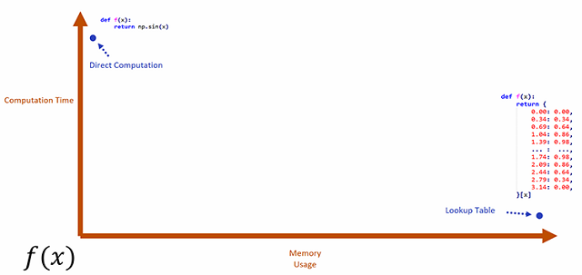
For example, let's consider a very simple Python program which computes sin(x):

def f(x):
    return np.sin(x)

This is what we would call a "direct" computation of the sin function, but let us imagine for a moment than the sin function was a very expensive operation to compute. In this case we might want to take a different approach. We could, for example, pre-compute values of sin(x) for many different values of x and store them in a big lookup table like follows:

def f(x):
    return {
        0.00: 0.00,
        0.34: 0.34,
        0.69: 0.64,
        1.04: 0.86,
        1.39: 0.98,
        ... :  ...,
        1.74: 0.98,
        2.09: 0.86,
        2.44: 0.64,
        2.79: 0.34,
        3.14: 0.00,
    }[x]

Now, instead of computing the value of sin(x) "directly" by some expensive operation, we can instead "compute" the value of sin(x) almost instantly by simply looking up the value of our input in the lookup table. The downside is this - now we need to pre-compute the sin function hundreds of thousands of times and keep all of those pre-computed values of sin(x) in memory. We have traded more memory usage (and pre-computation) in exchange for less computation. And, although the lookup table may become unfathomably huge, and the pre-computation time insanely large for complicated functions, in theory this very same trick is applicable to any function we are interested in - not just very simple functions like sin - functions even as complicated as a physics simulations.

We can think about these two programs like two extreme data points - two different ways to compute the same function with vastly different uses of computation and memory. If we were to measure their respective memory usage and computation time and plot them on a graph it would probably look something like this:

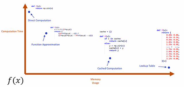
The natural question to ask next is if there are any generic programs which lie somewhere in-between these two extremes. Programs which trade off memory and computation in a way that is agnostic to the underlying function they are computing. In fact there are! We can, for example, write a generic program which caches computations to avoid re-computation. This saves some performance if we get an input we've already computed the output for at the cost of some additional memory usage:

cache = {}

def f(x):
    if x in cache:
        return cache[x]
    else:
        y = np.sin(x)
        cache[x] = y
        return y

Like before, we've found a "generic" way to trade-off memory for computation which can work (in theory at least) no matter what function we are interested in computing.

There are also programs that simply approximate the function we are interested in computing by using a bit more memory in exchange for faster and less accurate computation. Here is one such approximation for the sin function:

def f(x):
    x = x % (2*np.pi)
    return (
        (16*x*(np.pi - x)) / 
        (5*np.pi*np.pi - 4*x*(np.pi - x)))

It might not be clear at first where the additional memory usage in these functions is, but in this case the constants such as 2, 16, 5, 4, and pi are all additional "special" values, just like those in the lookup table - these are the "memory". And while this specific approximation is limited to sin, it isn't that difficult to find a generic version of this program which looks similar but can approximate any function simply by finding different appropriate constant values.

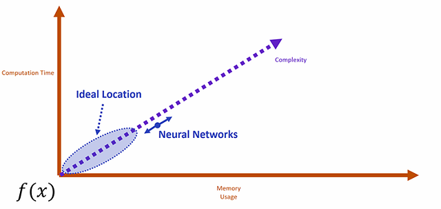
Given these two additions, another question to ask is this: Is there a generic kind of program like the ones we've presented so far which lies in the sweet spot at the bottom left of the graph - not using too much memory - not using too much computation - providing the best of both worlds?

One direction we can look towards is Machine Learning - because if we can evaluate the function we are interested in approximating offline we can gather training data and then train a generic Machine Learning algorithm to approximate the function. In Machine Learning we have a whole class of different generic algorithms we could add to our graph to see their performance.

As an example, let's take a look at Neural Networks - if we examine the computational properties of Neural Networks, we can probably guess where they might lie on this graph without even having to try them.

First of all, let's look at the computation time. Now, the computation time of a Neural Network is basically proportional to the number of weights it has, and the number of weights it has also dictates the memory usage. So computation time and memory usage are coupled in a standard Neural Network - visually, Neural Networks always lie somewhere on the diagonal of the graph.

And what dictates how many weights we need in a Neural Network? Well roughly, this is dictated by two things - how accurate we want the Neural Network to be, and how complex the function we are fitting is. If we look at all these properties together we see something like this

            Computation Time     is proportional to     Memory Usage
            Memory Usage         is proportional to     Accuracy
            Accuracy   is inversely proportional to     Complexity

So, how far up the diagonal our Neural Network will be is governed ultimately by the accuracy we want, and the complexity of the function we are interested in fitting. This is both good and bad news - good because if the function we want to approximate isn't complex then we can be confident we will hit the sweet spot - low computation time and low memory usage - and bad because if the function we want to approximate is complex we get the worst of both worlds - expensive evaluation and lots of memory usage.

But what exactly do we mean by the complexity of a function? If we could get a good intuitive understanding of this we would be able to predict more accurately when Neural Networks might hit the sweet spot. This is where Kolmogorov Complexity comes in - an intuitive measure for deciding how complex a function is.

---

Kolmogorov Complexity

Put simply, the Kolmogorov Complexity of some function is the length of the shortest possible program which can produce exactly the same outputs as the function for all given inputs. In addition, according to the rules of Kolmogorov Complexity, programs are not allowed to open any files or communicate with the outside world in any way - all their data must be stored in the source code.

For example, the function which takes no inputs and outputs the string:

abababababababababababababababab

can be produced pretty simply by the small program:

def f():
    print "ab" * 16

Which implies this function which outputs ab repeated is not a particularly complex function. On the other hand, the function which takes no inputs and produces the string:

4c1j5b2p0cv4w1x8rx2y39umgw5q85s7

is comparatively more complex - it basically requires a program to print out the string verbatim:

def f():
    print "4c1j5b2p0cv4w1x8rx2y39umgw5q85s7"

Storing this string makes the program much longer, which means the function which produces it must be complex.

There is already something interesting to note here - the first program computes something (using the * operator), while the second simply memorizes the string. This immediately gives us a good intuition: functions which need to do memorization are often more complex.

And Kolmogorov Complexity is not limited to functions which output strings. We can use exactly the same analysis for functions which produce images, physics simulations, or anything else. Consider the following images, do we think either of them are produced from complex functions?

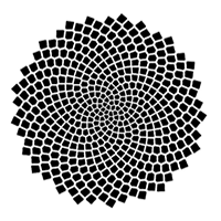
Well not really - probably there is a simple program which can produce either image - it looks like they took simple rules to generate. What about these images?

Now these are much more complex. It seems difficult to think of a program which could produce either of these images without storing lots of raw data inside the program. Here we gain another intuition: that natural data is often complex and requires memorization.

What about these two images?

Aha - this time it's a trick question. The first image is of course of a fractal - an image which appears complex but actually as we well know has a simple program that can be used to generate it.

The second is random noise - and can have two answers. If this noise is from a pseudo random number generator or we just want to produce noise but not this exact noise, it is technically not complex as we know that pseudo random number generators are relatively simple programs - however - if this is true random noise and we want to reproduce it exactly, then it is maximally complex - there is no possible program which could generate it without simply storing it verbatim and writing it out. This gives us another intuition: knowing the complexity of a function simply by observing its input and output is extremely difficult.

So what about something like a physics simulation? Forget about the edge cases and trick questions for now and imagine you had to write a program to produce the movement of the cloth in this video given the movement of the ball.

Is this complex?

Well...relative to our other examples certainly, but perhaps it isn't as complex as you might think at first - I think it would probably be possible to guess the motion of the cloth fairly accurately simply by knowing the phase of the movement of the ball. My gut feeling is that if you do something clever there may well be a simple program which could take just that one parameter and get a good guess at the state of the cloth in response.

What about this one?

Okay, now this is complex - there are all kind of tiny folds and chaotic movements going on and it would seem like you would need to write a massive complex program to produce this exact behavior.

But is there a way we can actually compute the complexity directly rather than just feeling around with our intuition? It has been shown that this is impossible in the general case - but we can compute an approximation of it with an algorithm called Principal Component Analysis (PCA). When you apply PCA to some data, what you get back is a guess at how many numbers might be required to express it for a given error threshold - a guess at how compressible the data is - and a simple algorithm for how to decompress it.

Let's try applying this to some data gathered from a physics simulation. Interestingly, when applied to physical simulation data, PCA has a special behavior - in addition to telling us the "complexity" of the simulation it also extracts the major axes of deformation for the physically simulated object we are interested in:

We can measure the complexity by looking at how many of these axes of deformation are required to reconstruct the original motion. For a simple motion like our sheet of cloth swinging back and forth we might only need one or two axes to almost entirely reconstruct the motion, while for our cloth with complex fine folds we could expect to need hundreds or even thousands.

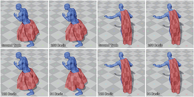
Below you can see a comparison of what happens if we choose different numbers of axes to reconstruct the movement of a cape attached to a character. With fewer axes you get less detail - the complexity is effectively reduced. In this case, although the original cloth has around 3000 vertices we need just 256 axes (sometimes also called Basis) to represent the state of the cloth without too much loss in quality, detail, and complexity.

This tells us something interesting - that physics simulations are almost always less complex than they may first appear (there is a good reason for this too, based on the theory of adding constraints). It tells us that if we try to approximate a fairly simple physics simulation with a Neural Network, we have a good chance of hitting the sweet spot between computation and memorization!

---

Squishy Bunnies

So let's try it - lets set up a bunch of simulations and run them for a long time to extract lots of different simulation data for some different situations we are interested in.

As you'd expect, extracting this kind of data can take a long time - up to several days - but once complete we have a massive database of physics simulation data we can learn from.

The next step is to apply PCA. At this point we can decide exactly how many axes we want to use by examining how well we can reproduce the original data. Fewer axes means fewer details, but also makes it much more likely we can hit the sweet spot in regards to performance.

Once we've applied PCA, for each frame we have N numbers, where N is the number of axes, each number representing the deformation on that axis. Using this representation, we want to train a Neural Network to predict the PCA values for the next frame, given the frame before, and the positions of all the different external objects such as the ball or whatever else.

In fact, we can ask the network to predict a correction to an extrapolation of the current deformation using the rate of change of the current deformation - in this case we get a more accurate prediction because most of the time objects change very consistently between frames.

Once trained, we can drop in our Neural Network as a replacement to the simulation function. And, while the normal physics simulation takes as input the full state of the cloth including all of the thousands of vertex positions - our network only takes as input just the N numbers representing the deformation on the PCA axes - and outputs the same. In this way it does vastly less computation and produces a much more efficient simulation.

And since the deformations computed from the PCA have a specific mathematical property (they are orthonormal), this exact formulation has a nice physical interpretation too - that under some basic assumptions we can say the Neural Network is actually being used to predict the forces applied in the simulation in a highly efficient way. Forces such as those introduced by collisions and internal tension. You can see the paper for more details.

Here you can see it applied to two small examples - a simple ball and sheet and a cloth pinned at four corners. At face value you would never know that behind the scenes no physics simulation is actually being performed - all of it is being approximated by a neural network!

We can also include as input to the network other things - such as the wind direction and speed. Here we can use it to control a flag:

What about a more complicated example? In this case the network gets as input the joint positions of the blue character and learns to predict the movement of the cape. It learns to do everything itself, including all of the collisions and other interaction dynamics. Here we can compare it to the ground truth simulation - we can see that while some details are lost, overall it does a pretty good job of approximating the result.

Here we plug it into an interactive system to see how it behaves in a more realistic environment.

It isn't just cloth, we can also approximate the deformation of soft bodies like this deformable bunny or this dragon. In these cases we get even more massive performance gains simply because simulating deformable objects is even more expensive.

If we adjust the number of PCA axes we use, we can also trade runtime performance and memory in exchange for quality (or we could say complexity in this case).

Naturally, our network only performs well on the kind of situations it's trained on. If we move the objects faster or further than what we had in the training data we don't get realistic behavior from the simulation:

Similarly, if we try to train it on situations which are too complex it simply takes too long to even get all the training data we need to cover every possible different situation we might be interested in covering. Additionally, if the complexity gets too high we hit the worst of both worlds - a massive neural network which requires huge amounts of memory and takes a long time to compute.

But as long as we remain in the range of the training data and the complexity is relatively low, we really can hit the sweet spot. Performance goes between 35us per frame, and 350us per frame - which is roughly within the budget for a character or other special entity in a AAA game production - and about 300 to 5000 times faster than the original simulation we used to get the training data. Having such fast performance also allows us to simulate a lot of things at once! Including things that would be totally impossible with normal simulation:

---

Conclusion

So Neural Networks are not just good for things we don't know how to solve, they can provide massive performance gains on problems we already know how to solve. In fact, we can use the concept of Kolmogorov Complexity to get a kind of intuition (and even use PCA for a simple kind of measure) for how well we expect Neural Networks to perform on a task.

But, thinking toward the future, there is still something awkward about all of this - which is that we didn't actually do what we originally wanted to do - which was to find a way to easily trade computation for memory usage and vice versa - in standard Neural Networks the two are coupled and computation time is always proportional to the number of weights. Yes, we can hit the sweet spot if the complexity is low, but what if it is high? Wouldn't it be nice to (for example) allow for a bit more memory usage to get computation time within a certain budget?

Wouldn't it be great in game development if we could adapt Neural Networks in a way which allowed us to set our budgets for computation and memory and have the result presented to us in whatever accuracy was possible. Recent research has shown some promising results, but it looks like we will have to wait a bit longer before that dream becomes a reality...