Pure Depth SSAO
21/10/2011
Edit (09/02/2025): This article is almost a decade and a half old now. At the time SSAO was a relatively new and unknown thing with not a lot of information online. While the implementation I shared here is far from one of the worst, it's also very heuristic and does not function in the view-space like it should. If you want some good, simple, correct implementations of various SSAO implementations including HBAO and others I suggest taking a look at the code from my NNAO paper instead.
Decided to finally take a look at some SSAO implementations. I was working in a pipeline that only had an early depth pass to generate it off so I was mainly looking at Crytek type implementations.
My final algorthm is heavily inspired by this one.
The main difference is just that my implementation is a little bit simpler, and a bit faster, with a few of the parts removed - though I don't think quality has been affected much. It also does not require normals data in a texture, but rather attempts to reconstruct it from the depth buffer when needed.
I also needed to tweak quite significantly a lot of the parameters. I ended up with some great results that look really quite similar to the Crytek implementation. Here are a couple of thoughts and things I learnt:
Randomness is really important. The noise texture is key and without it the algorthm result is barely recognizable as SSAO. When I disabled the randomness what I expected was a kind of 16-level banding (I was using 16 samples) but instead what I got was far from that. Only the darkest areas had a 16 layer banding. The rest, which was often only occluded by a couple of objects, got a kind of two or three tier banding. This banding was also far from regular - and more a consiquence of what particular sample directions were chosen. The main problem was that instead of a regular banding like you might get with PCF shadows, I actually got bands which were silhouettes of recognizable objects as well as all kinds of other very recognizable artifacts.
So the randomness is important. It isn't just a way of removing banding - I guess you can consider it sort of similar to the random variable in Monte Carlo integration.
When I finally realized how important the random factor was into the equation it still took a while to tweak the parameters until it was at a decent level. First results were very noisy and I wasn't really sure how to fix it. In fact it took me a long time to really work out how the different parameters effected the result. They can have some odd ranges and peculiar magnitudes for realistic values. Also don't assume you can just blindly copy the parameters from someone else's implementation. They are heavily dependant on factors such as the screen resolution and the near and far clipping planes.
Learning what they all do is key to getting the effect you want. There are many different kinds of effects and looks which are possible and most of them are a kind of trade off. In my final implementation I looked for a result which would really highlight and accentuate smaller details - the occlusion range looks like it is near to half a meter. The tradeoff for this look is that you can tend to get haloing and a kind of rim lighting around lots of objects. If you don't mind about the smaller details its perfectly possible to get an occlusion that looks much more like global illumination; though this often will halo in the opposite direction - putting shadows around objects which don't need it.
Unfortunately I was on a platform that didn't allow me to define uniforms which I could tweak with some sliders or something in-game - so I had to recompile the shaders every time with new constants. If you are given this opportunity to use some in-game value take it, because it will save you a whole lot of time.
Once you've tweaked the parameters to a good extent you'll probably be left with a somewhat noisy effect that generally looks like SSAO. With this you have a couple of options. What I would recommend is rendering it to texture, generating mipmaps and then using it down-sampled for whichever shaders you wish to apply the SSAO factor too. Most places also say that it should be applied to the ambient term but it can be interesting to play with it in other places too.
In the end my code looked something like this:
float3 normal_from_depth(float depth, float2 texcoords) {

  const float2 offset1 = float2(0.0,0.001);
  const float2 offset2 = float2(0.001,0.0);

  float depth1 = tex2D(DepthTextureSampler, texcoords + offset1).r;
  float depth2 = tex2D(DepthTextureSampler, texcoords + offset2).r;

  float3 p1 = float3(offset1, depth1 - depth);
  float3 p2 = float3(offset2, depth2 - depth);

  float3 normal = cross(p1, p2);
  normal.z = -normal.z;

  return normalize(normal);
}

PS_OUTPUT ps_ssao(VS_OUT_SSAO In)
{
  PS_OUTPUT Output;

  const float total_strength = 1.0;
  const float base = 0.2;

  const float area = 0.0075;
  const float falloff = 0.000001;

  const float radius = 0.0002;

  const int samples = 16;
  float3 sample_sphere[samples] = {
      float3( 0.5381, 0.1856,-0.4319), float3( 0.1379, 0.2486, 0.4430),
      float3( 0.3371, 0.5679,-0.0057), float3(-0.6999,-0.0451,-0.0019),
      float3( 0.0689,-0.1598,-0.8547), float3( 0.0560, 0.0069,-0.1843),
      float3(-0.0146, 0.1402, 0.0762), float3( 0.0100,-0.1924,-0.0344),
      float3(-0.3577,-0.5301,-0.4358), float3(-0.3169, 0.1063, 0.0158),
      float3( 0.0103,-0.5869, 0.0046), float3(-0.0897,-0.4940, 0.3287),
      float3( 0.7119,-0.0154,-0.0918), float3(-0.0533, 0.0596,-0.5411),
      float3( 0.0352,-0.0631, 0.5460), float3(-0.4776, 0.2847,-0.0271)
  };

  float3 random = normalize( tex2D(RandomTextureSampler, In.Tex0 * 4.0).rgb );

  float depth = tex2D(DepthTextureSampler, In.Tex0).r;

  float3 position = float3(In.Tex0, depth);
  float3 normal = normal_from_depth(depth, In.Tex0);

  float radius_depth = radius/depth;
  float occlusion = 0.0;
  for(int i=0; i < samples; i++) {

    float3 ray = radius_depth * reflect(sample_sphere[i], random);
    float3 hemi_ray = position + sign(dot(ray,normal)) * ray;

    float occ_depth = tex2D(DepthTextureSampler, saturate(hemi_ray.xy)).r;
    float difference = depth - occ_depth;

    occlusion += step(falloff, difference) * (1.0-smoothstep(falloff, area, difference));
  }

  float ao = 1.0 - total_strength * occlusion * (1.0 / samples);
  Output.RGBColor = saturate(ao + base);

  return Output;
}
Before I actually got into the nitty gritty details I always had trouble trying to imagine how SSAO algorithms worked. The trouble was in all the articles I had read they talked about a "sampling sphere" and I began to assume that it required a fully deferred pipeline with position data in a buffer as well as all kinds of other stuff. In reality it is far more simple. It does have a sampling sphere but this is a purely screen-space construct and you can imagine it in a flattened context most of the time. The reason for this - rather than say a sampling circle - is to ensure the sampling density is correctly distributed in the space.
The basic idea is this. For each pixel imagine this sampling sphere. In this sphere we generate 16 random vectors. We then work out the screen-space normal of the initial pixel. It is good to also imagine this normal being represented in the same sampling sphere. All the vectors which are pointing in the opposite direction to the normal we flip so that now they are in the same hemisphere as the normal vector.
These vectors act as our samples. We simply project each of them back onto the depth texture and look at the depth they point at. If the depth is closer to the viewer than the initial pixel's depth then we record the initial pixel as being occluded by some amount.
To work out the amount of occlusion you can use various methods. Ideally you want some difference to be the perfect occlusion, with a larger or smaller depth difference meaning less occlusion. We can represent this quite nicely using the smoothstep function and it also gives us a good boundary so we know when pixels are absolutely not occluded by another.
With this image in my head it is clear to see how it works. A surface effectively looks in front of itself for any pixels which might overshadow it. Imagine a pixel on a ground surface almost perpendicular to the screen. It will generate a hemisphere which points upwards in screen space and sample pixels almost directly above it. This is almost precisely what we need for occlusion - and why the simple algorithm is so effective.
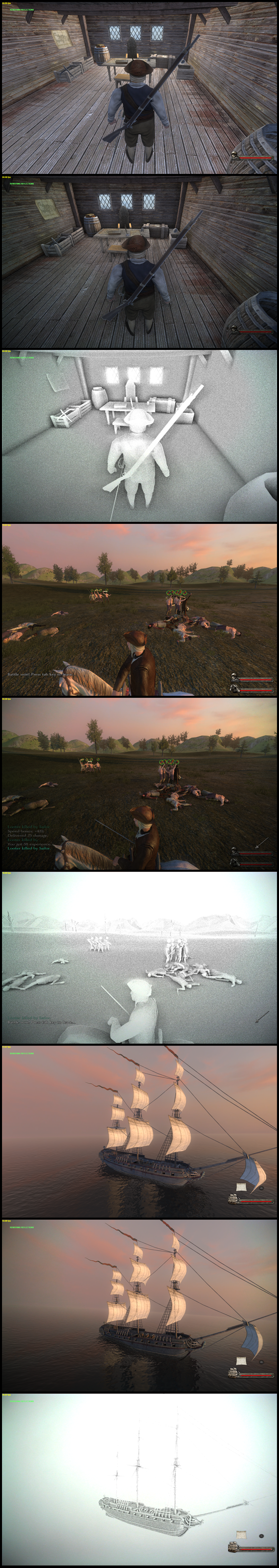
Anyway, please use/borrow/steal the above code for whatever needs you have. If you have any questions feel free to drop me an e-mail. Here are some pictures of the results: