Cubic Interpolation of Quaternions
25/04/2023
If you've ever googled "cubic interpolation of quaternions" or looked up the "SQUAD" algorithm you'd be forgiven for thinking that understanding how to do smooth, cubic interpolation of quaternions requires some really advanced mathematics.
But it really doesn't need to be that complicated. And if we understand well the algorithm for normal cubic interpolation (and more specifically, Catmull-Rom cubic interpolation), the quaternion version pretty much falls into our laps.
Whenever the subject of cubic interpolation and splines comes up it would be wrong of me not to recommend the absolute master-class that is Freya Holmer's spline videos - watching these should give you a great intuition not just about the process we are going to go through in this article, but about splines in general.
Hermite Curve Interpolation
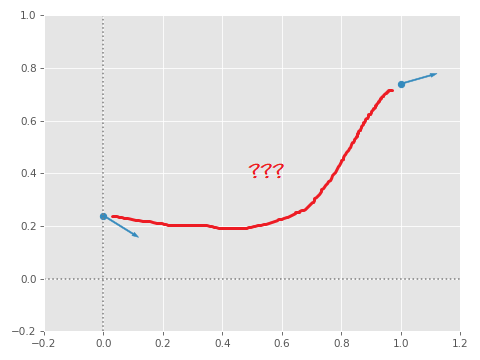
Forget about quaternions for now. Instead, we're going to start with the following more simple problem: if we have two values at 0 and 1, and gradients for those values at 0 and 1, how can we produce a smooth interpolation which passes through those values with the given gradients?
The solution is to fit a cubic polynomial function \( f \) to the two points and their gradients. In this case we have four constraints...
\begin{align*} f(0) &= p_0 \\ f(1) &= p_1 \\ f'(0) &= v_0 \\ f'(1) &= v_1 \\ \end{align*}
...and four unknowns \( a \), \( b \), \( c \), and \( d \).
\begin{align*} f(x) &= a\ x^3 + b\ x^2 + c\ x + d \\ f'(x) &= 3\ a\ x^2 + 2\ b\ x + c \\ \end{align*}
So we just need to plug our different equations into each other and solve for \( a \), \( b \), \( c \), and \( d \).
First we solve for \( d \) using our first constraint \( f(0) = p_0 \)...
\begin{align*} p_0 &= a\ 0 + b\ 0 + c\ 0 + d \\ d &= p_0 \\ \end{align*}
Then we solve for \( c \) using our third constraint \( f'(0) = v_0 \)...
\begin{align*} v_0 &= 3\ a\ 0 + 2\ b\ 0 + c \\ c &= v_0 \\ \end{align*}
Then we can solve for \( b \) using our other two constraints and our solutions for \( d \) and \( c \)...
\begin{align*} p_1 &= a\ 1 + b\ 1 + c\ 1 + d \\ a &= p_1 - b - v_0 - p_0 \\ &\\ v_1 &= 3\ a\ 1 + 2\ b\ 1 + c \\ v_1 &= 3\ (p_1 - b - v_0 - p_0) + 2\ b + v_0 \\ v_1 &= 3\ p_1 - 3\ b - 3\ v_0 - 3\ p_0 + 2\ b + v_0 \\ b &= 3\ p_1 - 2\ v_0 - 3\ p_0 - v_1 \\ \end{align*}
And finally we can solve for \( a \)...
\begin{align*} a &= p_1 - b - v_0 - p_0 \\ a &= p_1 - (3\ p_1 - 2\ v_0 - 3\ p_0 - v_1) - v_0 - p_0 \\ a &= v_0 + 2\ p_0 + v_1 - 2\ p_1 \\ \end{align*}
We can plot this cubic function to verify that it passes through the given points, and with the correct gradients:
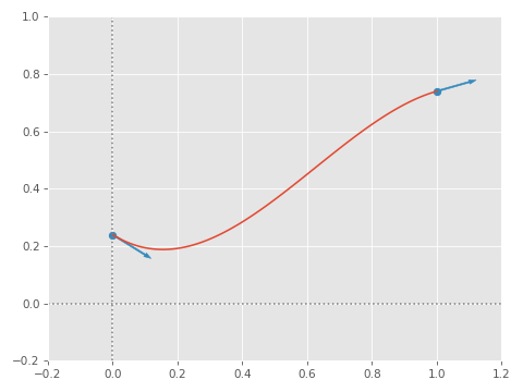
Nice! If we expand the cubic function with our values for \( a \), \( b \), \( c \), and \( d \) substituted, we can rearrange things such that our result is expressed in terms of \( p_0 \), \( p_1 \), \( v_0 \) and \( v_1 \) directly (rather than the polynomial coefficients):
\begin{align*} f(x) &= (v_0 + 2\ p_0 + v_1 - 2\ p_1)\ x^3 + (3\ p_1 - 2\ v_0 - 3\ p_0 - v_1)\ x^2 + v_0\ x + p_0 \\ f(x) &= v_0\ x^3 + 2\ p_0\ x^3 + v_1\ x^3 - 2\ p_1\ x^3 + 3\ p_1\ x^2 - 2\ v_0\ x^2 - 3\ p_0\ x^2 - v_1\ x^2 + v_0\ x + p_0 \\ f(x) &= p_0\ (2\ x^3 - 3\ x^2 + 1) + p_1\ (3\ x^2 - 2\ x^3) + v_0\ (x^3 - 2\ x^2 + x) + v_1\ (x^3 - x^2) \\ \end{align*}
This is useful because usually \( x \) is a scalar, while \( p_0 \), \( p_1 \), \( v_0 \) and \( v_1 \) can often be 3d vectors. For example, we can implement a version that works on 3d vectors in C++ as follows, where x is our interpolating value between 0 and 1:
vec3 hermite_basic(float x, vec3 p0, vec3 p1, vec3 v0, vec3 v1)
{
    float w0 = 2*x*x*x - 3*x*x + 1;
    float w1 = 3*x*x - 2*x*x*x;
    float w2 = x*x*x - 2*x*x + x;
    float w3 = x*x*x - x*x;

    return w0*p0 + w1*p1 + w2*v0 + w3*v1;
}
(Aside: Notice how w0 and w1 are both versions of smoothstep - isn't that cool!)
Since we have the derivative of our cubic polynomial function, we can also compute the gradient/velocity of the interpolated result and get our function to output that too:
void hermite(
    vec3& pos,
    vec3& vel,
    float x,
    vec3 p0,
    vec3 p1,
    vec3 v0,
    vec3 v1)
{
    float w0 = 2*x*x*x - 3*x*x + 1;
    float w1 = 3*x*x - 2*x*x*x;
    float w2 = x*x*x - 2*x*x + x;
    float w3 = x*x*x - x*x;

    float q0 = 6*x*x - 6*x;
    float q1 = 6*x - 6*x*x;
    float q2 = 3*x*x - 4*x + 1;
    float q3 = 3*x*x - 2*x;

    pos = w0*p0 + w1*p1 + w2*v0 + w3*v1;
    vel = q0*p0 + q1*p1 + q2*v0 + q3*v1;
}
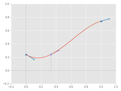
Which looks something like this:
One last adjustment to this formula is to effectively translate our points such that \( p_0 = 0 \). Then, once we have the interpolated value, translate it back up by adding the original value of \( p_0 \):
void hermite_alt(
    vec3& pos,
    vec3& vel,
    float x,
    vec3 p0,
    vec3 p1,
    vec3 v0,
    vec3 v1)
{
    vec3 p1_sub_p0 = p1 - p0;

    float w1 = 3*x*x - 2*x*x*x;
    float w2 = x*x*x - 2*x*x + x;
    float w3 = x*x*x - x*x;

    float q1 = 6*x - 6*x*x;
    float q2 = 3*x*x - 4*x + 1;
    float q3 = 3*x*x - 2*x;

    pos = w1*p1_sub_p0 + w2*v0 + w3*v1 + p0;
    vel = q1*p1_sub_p0 + q2*v0 + q3*v1;
}
This might seem like a pointless extra step, but this formulation with the first point at zero actually simplifies things in a way which will be really useful when we start dealing with quaternions.
What we've derived is called Hermite Cubic Interpolation, and is essentially the mathematics used for a single segment of a Hermite Spline, which will be a key part of doing cubic interpolation of quaternions.
Catmull-Rom Cubic Interpolation
If we have a series of points and their gradients/velocities, we can use the previous equation to make a smooth interpolation that passes through them. But what if we just have points? With no velocities or gradients associated with them? Can we still use Hermite Curve Interpolation?
Yes! The trick is to take four points instead of two, and to use the central difference to "estimate" a gradient/velocity to associate with each of the middle two points. Then, once we have these velocities we can use Hermite Curve Interpolation to interpolate the intermediate values.
In code it looks something like this:
void catmull_rom(
    vec3& pos,
    vec3& vel,
    float x,
    vec3 p0,
    vec3 p1,
    vec3 p2,
    vec3 p3)
{
    vec3 v1 = ((p1 - p0) + (p2 - p1)) / 2;
    vec3 v2 = ((p2 - p1) + (p3 - p2)) / 2;
    hermite(pos, vel, x, p1, p2, v1, v2);
}
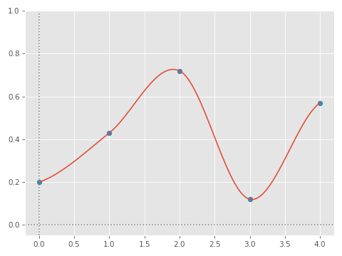
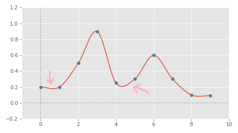
You can see that we compute the central difference for these two middle points using the average of the forward and backward differences. Then, we pass these estimated velocities to our Hermite Curve Interpolation function to get the final interpolated value! The result is something like this:
And that's how we use a Catmull-Rom spline to do cubic interpolation. Here is what it looks like in 3d:
Quaternion Catmull-Rom Cubic Interpolation
Now that we understand exactly what is going on (and what each different value and computation represents) we are ready to adapt our equations to work with quaternions instead of positions.
First we will tackle the Hermite Cubic Interpolation function, and there are a few changes we need to make to get this formula to work for quaternions:
- Instead of linear velocities, we need to use angular velocities.
- When we compute the difference between
p0andp1to putp0at zero, we are instead going to take the quaternion difference. - Once we have this quaternion difference, we are going to convert it into the scaled-angle-axis space so that it makes sense to mix it with angular velocities.
- Once we have added everything together, we need to convert the result back to a quaternion. And instead of adding back the original value of
p0we will use quaternion multiplication.
In code it looks like this:
void quat_hermite(
    quat& rot,
    vec3& vel,
    float x,
    quat r0,
    quat r1,
    vec3 v0,
    vec3 v1)
{
    float w1 = 3*x*x - 2*x*x*x;
    float w2 = x*x*x - 2*x*x + x;
    float w3 = x*x*x - x*x;

    float q1 = 6*x - 6*x*x;
    float q2 = 3*x*x - 4*x + 1;
    float q3 = 3*x*x - 2*x;

    vec3 r1_sub_r0 = quat_to_scaled_angle_axis(quat_abs(quat_mul_inv(r1, r0)));

    rot = quat_mul(quat_from_scaled_angle_axis(w1*r1_sub_r0 + w2*v0 + w3*v1), r0);
    vel = q1*r1_sub_r0 + q2*v0 + q3*v1;
}
Next, we can tackle our Catmull-Rom Cubic Interpolation function. This time there are fewer adjustments. All we really need to do is convert our velocity computations via finite difference, into angular velocity computations via finite difference (as described in my previous article on angular velocity)...
void quat_catmull_rom(
    quat& rot,
    vec3& vel,
    float x,
    quat r0,
    quat r1,
    quat r2,
    quat r3)
{
    vec3 r1_sub_r0 = quat_to_scaled_angle_axis(quat_abs(quat_mul_inv(r1, r0)));
    vec3 r2_sub_r1 = quat_to_scaled_angle_axis(quat_abs(quat_mul_inv(r2, r1)));
    vec3 r3_sub_r2 = quat_to_scaled_angle_axis(quat_abs(quat_mul_inv(r3, r2)));

    vec3 v1 = (r1_sub_r0 + r2_sub_r1) / 2;
    vec3 v2 = (r2_sub_r1 + r3_sub_r2) / 2;
    quat_hermite(rot, vel, x, r1, r2, v1, v2);
}
And that's it! While some of these steps might not be 100% obvious without thinking about it a little, as long as you understand the relationship between angular velocities and quaternions, I don't think there is anything unexpected going on.
Here is what it looks like in our little 3d environment:
Raw Quaternion Cubic Interpolation
If you are interpolating a series of quaternions which are sequentially pretty similar to each other, and have been "unrolled" so that there are no sudden discontinuities there is an even easier way to do cubic interpolation of quaternions, which is to just do the interpolation directly in the 4d quaternion space, treating the quaternions as 4d vectors, and re-normalize the result.
This can be faster and will produce practically identical results when your quaternions are similar. I see this as like the difference between using slerp and nlerp for linear interpolation.
One thing to be careful of in this setup is that if you are treating the quaternions as raw 4d vectors then the "velocities" you get out of the cubic interpolation will not be angular velocities, but velocities in the raw 4d quaternion space.
If we want to convert these "velocities" in the 4d quaternion space into actual angular velocities we can do so using the following function:
vec3 quat_delta_to_angular_velocity(quat qref, quat qdelta)
{
    quat a = quat_mul_inv(qdelta, qref);
    return 2.0f * vec3(a.x, a.y, a.z);
}
Here qdelta is the scaled raw difference between two quaternions in the 4d space and qref is a quaternion representing the rotation at which this difference was taken (i.e. one of the two quaternions used to compute the difference or the rotation along the spline associated with this difference).
This gives a result equal to the linear approximation of the angular velocity.
Conclusion
When it comes to animation data, I think most people believe that doing cubic interpolation of rotations is a waste of CPU cycles. Yes - sampling four poses is more expensive than two and the mathematics involved are more expensive too - but cubic interpolation really can make a visual difference - in particular when playing animation in slow-motion.
In addition, compared to linear interpolation, cubic interpolation gives velocities that change smoothly in-between frames, which can prevent aliasing effects when further processing the data. For example, sampling velocities for a motion-matching database via linear interpolation at a rate higher than the original animation data will produce consecutive entries with the same velocities - which can look like a bug when it comes to inspect the data and can affect the result of downstream algorithms such as PCA.
Here is another concrete example: while FIFA 21 has undoubtedly some of the best, most sophisticated, and most realistic animation in the world of video games, the linear interpolation between frames, and the velocity discontinuity this introduces during slow-mo is something that cannot be un-seen.
Edit: FIFA 23 on the other hand does use a similar technique to the one described here. I think the results speak for themselves!
Either way, I hope this post has shed some light on cubic interpolation of quaternions. And as always, thanks for reading!
Appendix: Cubic Interpolation of Scales
Those of you who have read my article on scalar velocity will know that we can follow a very similar process to derive a method of cubic interpolation of scales.
Again, we can start with a function for a hermite spline, this time taking scalar velocities as input (for this code, using the natural base).
void scale_hermite(
    vec3& scl,
    vec3& svl,
    float x,
    vec3 s0,
    vec3 s1,
    vec3 v0,
    vec3 v1)
{
    float w1 = 3*x*x - 2*x*x*x;
    float w2 = x*x*x - 2*x*x + x;
    float w3 = x*x*x - x*x;

    float q1 = 6*x - 6*x*x;
    float q2 = 3*x*x - 4*x + 1;
    float q3 = 3*x*x - 2*x;

    vec3 s1_sub_s0 = log(s1 / s0);

    scl = exp(w1*s1_sub_s0 + w2*v0 + w3*v1) * s0;
    svl = q1*s1_sub_s0 + q2*v0 + q3*v1;
}
Then, the catmull-rom derivation follows in exactly the same way - with scalar velocities computed as shown previously.
void scale_catmull_rom(
    vec3& scl,
    vec3& svl,
    float x,
    vec3 s0,
    vec3 s1,
    vec3 s2,
    vec3 s3)
{
    vec3 s1_sub_s0 = log(s1 / s0);
    vec3 s2_sub_s1 = log(s2 / s1);
    vec3 s3_sub_s2 = log(s3 / s2);

    vec3 v1 = (s1_sub_s0 + s2_sub_s1) / 2;
    vec3 v2 = (s2_sub_s1 + s3_sub_s2) / 2;
    scale_hermite(scl, svl, x, s1, s2, v1, v2);
}
And this is what it looks like in action:
Appendix: Preventing Overshoot
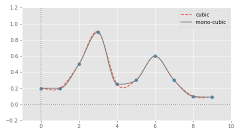
One of the big problems with cubic interpolation for animation data is that you can get over-shooting effects:
When you have an abrupt stop, this can result in the movement of the character extrapolating beyond the keyframe, and then returning back, all within the interpolation period.
Luckily there is a very simple solution to this called monotone cubic interpolation, which is detailed beautifully in a fantastic blog post by James Bird.
I highly suggest reading James' blog post for all the details, but the basic idea is this: to ensure that the interpolation never overshoots, there are some simple heuristics we can apply to constrain the velocities we pass to the hermite spline interpolation function.
More specifically there are two constraints we need to apply. First, if the two velocities that are averaged are in opposite directions then the velocity associated with that spline point must be zero instead. Second, the magnitude of the velocity for the spline point must never exceed three times the magnitude of either of the individual two averaged velocities.
This can be implemented quite straight-forwardly as follows. First, here for positions:
float cubic_mono_velocity(float d0, float d1)
{
    return signf(d0) != signf(d1) ? 0.0f : clampf(
        (d0 + d1) / 2,
        maxf(-3.0f * fabsf(d0), -3.0f * fabsf(d1)),
        minf(+3.0f * fabsf(d0), +3.0f * fabsf(d1)));
}

vec3 cubic_mono_velocity(vec3 d0, vec3 d1)
{
    return vec3(
        cubic_mono_velocity(d0.x, d1.x),
        cubic_mono_velocity(d0.y, d1.y),
        cubic_mono_velocity(d0.z, d1.z));
}

void catmull_rom_mono(
    vec3& pos,
    vec3& vel,
    float x,
    vec3 p0,
    vec3 p1,
    vec3 p2,
    vec3 p3)
{
    vec3 d10 = p1 - p0;
    vec3 d21 = p2 - p1;
    vec3 d32 = p3 - p2;

    vec3 v1 = cubic_mono_velocity(d10, d21);
    vec3 v2 = cubic_mono_velocity(d21, d32);
    return hermite(pos, vel, x, p1, p2, v1, v2);
}
And here for rotations:
void quat_catmull_rom_mono(
    quat& rot,
    vec3& vel,
    float x,
    quat r0,
    quat r1,
    quat r2,
    quat r3)
{
    vec3 d10 = quat_to_scaled_angle_axis(quat_abs(quat_mul_inv(r1, r0)));
    vec3 d21 = quat_to_scaled_angle_axis(quat_abs(quat_mul_inv(r2, r1)));
    vec3 d32 = quat_to_scaled_angle_axis(quat_abs(quat_mul_inv(r3, r2)));

    vec3 v1 = cubic_mono_velocity(d10, d21);
    vec3 v2 = cubic_mono_velocity(d21, d32);
    return quat_hermite(rot, vel, x, r1, r2, v1, v2);
}
And finally for scales:
void scale_catmull_rom_mono(
    vec3& scl,
    vec3& svl,
    float x,
    vec3 s0,
    vec3 s1,
    vec3 s2,
    vec3 s3)
{
    vec3 d10 = log(s1 / s0);
    vec3 d21 = log(s2 / s1);
    vec3 d32 = log(s3 / s2);

    vec3 v1 = cubic_mono_velocity(d10, d21);
    vec3 v2 = cubic_mono_velocity(d21, d32);
    return scale_hermite(scl, svl, x, s1, s2, v1, v2);
}
Here is what the result looks like in 1D compared to normal cubic interpolation.
And here is what it looks like in 3D:
This always ensures that the interpolated result lies within the domain of the data points, but still produces smooth interpolations and continuously varying velocities.