Fitting Code Driven Displacement Revisited
15/02/2026
One of Epic's very talented technical animators Maksym Zhuravlov recently came to me with some interesting spring-movement-model-related maths questions.
Obviously this was right up my street and I thought it could be nice to share my investigations.
The first question is this: if we have a character's movement driven by a critical spring damper, can we estimate how long it will take the character to stop and start, and can we estimate how far they will travel during those times?
And, perhaps an even more interesting follow up: if that is possible, then given some measurements for starting and stopping times and distances, can we estimate the spring parameters that best model those movements?
The answer turns out to be yes under some basic assumptions and with some interesting mathematics involved.
Stopping Distance
Let's start with how to estimate stopping distances. First a recap: if we have a character driven by a critical spring damper, that means the velocity of the character is updated for a delta-time of \( t \) using the following equation:
\begin{align*} v_{t} &= j_0 \cdot e^{-y \cdot t} + t \cdot j_1 \cdot e^{-y \cdot t} + c \\ \end{align*}
where
\begin{align*} j_0 &= v_0 - c \\ j_1 &= a_0 + j_0 \cdot y \\ \end{align*}
and \( v_t \) is the velocity of the character after time \( t \), \( v_0 \) is the current velocity, \( a_0 \) is the current acceleration, \( c \) is the target velocity, and \( y \) is the half-damping.
That means if we want to compute the stopping distance, we need to compute something like the absolute value of the integral of this equation with respect to time \( t \) from \( 0 \) to \( \infty \), when the target velocity \( c \) is \( 0 \):
The indefinite integral of the previous equation is as follows:
\begin{align*} x_{t} &= \int (j_0 \cdot e^{-y \cdot t} + t \cdot j_1 \cdot e^{-y \cdot t} + c) dt \\ x_{t} &= \tfrac{-j_1}{y^2} \cdot e^{-y \cdot t} + \tfrac{-j_0 - j_1 \cdot t}{y} \cdot e^{-y \cdot t} + \tfrac{j_1}{y^2} + \tfrac{j_0}{y} + c \cdot t + x_0 \\ \end{align*}
And here is what we get for distance \( d \) if we plug in \( c = 0\) and integrate from \( t = 0 \) to \( t = \infty \):
\begin{align*} d &= (\tfrac{-j_1}{y^2} \cdot e^{-y \cdot \infty} + \tfrac{-j_0 - j_1 \cdot \infty}{y} \cdot e^{-y \cdot \infty} + \tfrac{j_1}{y^2} + \tfrac{j_0}{y} + 0 \cdot \infty)\\ &- (\tfrac{-j_1}{y^2} \cdot e^{-y \cdot 0} + \tfrac{-j_0 - j_1 \cdot 0}{y} \cdot e^{-y \cdot 0} + \tfrac{j_1}{y^2} + \tfrac{j_0}{y} + 0 \cdot 0) \\ d &= (\tfrac{j_1}{y^2} + \tfrac{j_0}{y}) - (\tfrac{-j_1}{y^2} + \tfrac{-j_0}{y} + \tfrac{j_1}{y^2} + \tfrac{j_0}{y}) \\ d &= \tfrac{j_1}{y^2} + \tfrac{j_0}{y} \\ d &= \tfrac{a_0 + v_0 \cdot y}{y^2} + \tfrac{v_0}{y} \\ d &= \tfrac{a_0 + 2 \cdot v_0 \cdot y}{y^2} \\ \end{align*}
We do need to be careful though. As I noted in a previous article with a very similar derivation, this doesn't actually give us the distance exactly, since it will count areas under the x-axis as negative and above the x-axis as positive:
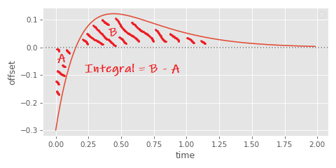
So if we want the distance travelled we need to find if there is an intersection time and if so solve the integral in two parts. The intersection time can be computed as follows:
\begin{align*} v_t &= j_0 \cdot e^{-y \cdot t} + t \cdot j_1 \cdot e^{-y \cdot t} + c \\ 0 &= (j_0 + t \cdot j_1) \cdot e^{-y \cdot t} + 0 \\ 0 &= v_0 + t \cdot (a_0 + j_0 \cdot y) \\ t &= \frac{-v_0}{a_0 + v_0 \cdot y} \\ \end{align*}
And the integral from \( 0 \) to \( t \) can be derived as follows:
\begin{align*} d &= (\tfrac{-j_1}{y^2} \cdot e^{-y \cdot t} + \tfrac{-j_0 - j_1 \cdot t}{y} \cdot e^{-y \cdot t} + \tfrac{j_1}{y^2} + \tfrac{j_0}{y} + 0 \cdot t)\\ &- (\tfrac{-j_1}{y^2} \cdot e^{-y \cdot 0} + \tfrac{-j_0 - j_1 \cdot 0}{y} \cdot e^{-y \cdot 0} + \tfrac{j_1}{y^2} + \tfrac{j_0}{y} + 0 \cdot 0) \\ d &= (\tfrac{-j_1}{y^2} \cdot e^{-y \cdot t} + \tfrac{-j_0 - j_1 \cdot t}{y} \cdot e^{-y \cdot t} + \tfrac{j_1}{y^2} + \tfrac{j_0}{y}) - (\tfrac{-j_1}{y^2} + \tfrac{-j_0}{y} + \tfrac{j_1}{y^2} + \tfrac{j_0}{y}) \\ d &= \tfrac{-(a_0 + v_0 \cdot y)}{y^2} \cdot e^{-y \cdot t} + \tfrac{-v_0 - (a_0 + v_0 \cdot y) \cdot t}{y} \cdot e^{-y \cdot t} + \tfrac{a_0 + v_0 \cdot y}{y^2} + \tfrac{v_0}{y} \\ d &= \tfrac{a_0 + 2 \cdot v_0 \cdot y}{y^2} - \tfrac{e^{-y \cdot t}}{y^2} \cdot (t \cdot a_0 \cdot y + v_0 \cdot y \cdot (t \cdot y + 2) + a_0) \\ \end{align*}
Which we can then use to compute the distance correctly. In code it looks like this:
def character_inflection_time(
    v,        # Initial Velocity
    a,        # Initial Acceleration
    halflife, # Halflife
    ):

    y = halflife_to_damping(halflife) / 2.0

    return -v / (a + v*y)

def character_stopping_distance(
    v,        # Initial Velocity
    a,        # Initial Acceleration
    halflife, # Halflife
    ):

    y = halflife_to_damping(halflife) / 2.0

    t = character_inflection_time(v, a, halflife)

    i0 = (v*y*2 + a) / (y * y)
    it = (np.exp(-y*t) / (y*y)) * (t*a*y + v*y*(t*y+2) + a)

    return np.where(t > 0.0, abs(i0 - it) + abs(it), abs(i0))
This computes the stopping distance accurately, but there is another simplification that is useful. If we assume the initial acceleration of the character \( a_0 \) is zero then we can be certain there is never any intersection of the x-axis, and all of this simplifies down much further:
\begin{align*} d &= \frac{a_0 + 2 \cdot v_0 \cdot y}{y^2} \\ d &= \frac{0 + 2 \cdot v_0 \cdot y}{y^2} \\ d &= \frac{2 \cdot v_0}{y} \\ \end{align*}
Which in code it looks like this:
def character_stopping_distance_approx(
    v,        # Initial Velocity
    halflife, # Halflife
    ):

    y = halflife_to_damping(halflife) / 2.0

    return np.abs(2*v / y)
Now, if we want to estimate the half-life from the stopping distance we can simply re-arrange this equation in terms of \( y \) instead:
\begin{align*} d &= \frac{2 \cdot v_0}{y} \\ y &= \frac{2 \cdot v_0}{d} \\ \end{align*}
Which in code simplifies to this:
def character_halflife_from_stopping_distance(
    v,        # Initial Velocity
    d,        # Distance
    ):

    return damping_to_halflife(4.0*v / d)
Which finally allows us to estimate a spring half-life from a stopping distance. Nice!
Stopping Time
What about stopping time? Well, this one is more tricky. The first issue is this: what exactly do we mean by stopping time? In mathematical terms, our spring never actually reaches the target velocity exactly - it only exponentially approaches it. So mathematically at least, we never actually really come to a complete stop!
A practical solution is to define the stopping time as the time at which the character velocity goes below some threshold. Then, if we take take another look at our critical spring equation from earlier we can see it already relates velocity of the character at some time \( v_t \) to the target velocity \( c \), the time \( t \), half-damping \( y \), and initial velocity \( v_0 \) and acceleration \( a_0 \):
\begin{align*} v_{t} &= (v_0 - c) \cdot e^{-y \cdot t} + t \cdot (a_0 + (v_0 - c) \cdot y) \cdot e^{-y \cdot t} + c \\ \end{align*}
So if we were to set \( v_t \) to some small value between \( v_t \) and \( 0 \) we'll call \( \epsilon \) and solve for \( t \), in theory this should give us how long it takes to come to an (almost) stop.
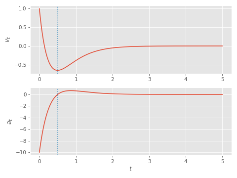
Well... kind of. The first problem is that, just as we saw before, if the initial acceleration is large, the character might hit our velocity target \( \epsilon \) but overshoot and continue to take a while to really come to a stop:
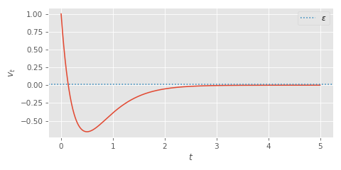
So if this approach is going to work we are going to need to assume the character always begins their stop with zero acceleration:
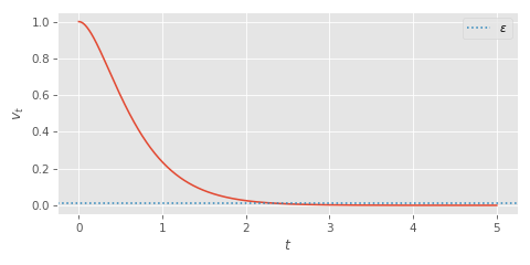
We can make another simplifying assumption. We can observation that the total vertical scale doesn't change how long it takes for the spring to reach the target (as noted here). So if we solve for the case where \( v_0 = 1 \), \( c = 0 \), \( a_0 = 0 \) this actually generalises to any other initial velocity \( v_0 \). We just need to scale the threshold \( \epsilon \) appropriately.
So substituting those values into our spring equation, it simplifies to the following:
\begin{align*} v_{t} &= (v_0 - c) \cdot e^{-y \cdot t} + t \cdot (a_0 + (v_0 - c) \cdot y) \cdot e^{-y \cdot t} + c \\ \epsilon &= (1 - 0) \cdot e^{-y \cdot t} + t \cdot (0 + (1 - 0) \cdot y) \cdot e^{-y \cdot t} + 0 \\ \epsilon &= e^{-y \cdot t} + t \cdot y \cdot e^{-y \cdot t} \\ \epsilon &= (1 + (t \cdot y)) \cdot e^{-y \cdot t} \\ \end{align*}
Unfortunately this still isn't so easy to solve for \( t \). The issue is that \( t \) appears both in the exponential multiplier \( (1 + (t \cdot y)) \) and in the power \( -y \cdot t \). To solve this equation for \( t \) we need to use something that was entirely new to me when I started looking at this - called the Lambert W function or product logarithm.
Very briefly, this function lets you take an equation of the form:
\begin{align*} ae^a &= b \\ \end{align*}
And transform it into the form:
\begin{align*} a &= W(b) \\ \end{align*}
Where \( W \) is the aforementioned product logarithm function. This means we need to re-arrange our equation so it looks something like \( ae^a = b \).
If we fiddle around a bit, eventually we can find that this can be done as follows:
\begin{align*} \epsilon &= (1 + (t \cdot y)) \cdot e^{-y \cdot t} \\ -\epsilon &= (-1 - (y \cdot t)) \cdot e^{-y \cdot t} \\ -\tfrac{\epsilon}{e} &= (-1 - (y \cdot t)) \cdot e^{-1 - y \cdot t} \\ \end{align*}
Now we can use the product logarithm to solve for \( t \):
\begin{align*} -\tfrac{\epsilon}{e} &= (-1 - (y \cdot t)) \cdot e^{-1 - y \cdot t} \\ W(-\tfrac{\epsilon}{e}) &= -1 - (y \cdot t) \\ W(-\tfrac{\epsilon}{e}) + 1 &= - (y \cdot t) \\ -\frac{W(-\tfrac{\epsilon}{e}) + 1}{y} &= t \\ \end{align*}
In python you can access the Lambert W function via scipy.special.lambertw. And for this case we need to take the -1 branch. Here is how it looks in code:
from scipy.special import lambertw

def character_stopping_time(
    v,        # Initial Velocity
    halflife, # Halflife
    v_eps,    # Velocity Threshold
    ):

    y = halflife_to_damping(halflife) / 2.0

    v_scale = v_eps / v

    return -(lambertw(-v_scale / np.e, -1).real + 1) / y
The product logarithm function is not in the standard C math library. But luckily, it isn't too difficult to implement a simplified version specialized to the -1 branch that is sufficient for our needs. I found a very nice implementation that works perfectly here:
float lambert_wm1f(const float x)
{
    if (isnan(x)) { return NAN; }
    if (x == 0.0f) { return -INFINITY; }
    if (x > 0.0f) { return NAN; }

    const float em1_fact_0 = 0.625529587f;
    const float em1_fact_1 = 0.588108778f;
    const float redx = em1_fact_0 * em1_fact_1 + x;

    if (redx <= 0.09765625f)
    {
        float r = sqrtf(redx);
        float w =  -3.30250000e+2f;
        w = w * r + 3.53563141e+2f;
        w = w * r - 1.91617889e+2f;
        w = w * r + 4.94172478e+1f;
        w = w * r - 1.23464909e+1f;
        w = w * r - 1.38704872e+0f;
        w = w * r - 1.99431837e+0f;
        w = w * r - 1.81044364e+0f;
        w = w * r - 2.33166337e+0f;
        w = w * r - 1.00000000e+0f;
        return w;
    }
    else
    {
        const float c0 =  1.68090820e-1f;
        const float c1 = -2.96497345e-3f;
        const float c2 = -2.87322998e-2f;
        const float c3 =  7.07275391e-1f;
        const float ln2 = 0.69314718f;
        const float l2e = 1.44269504f;

        const float s = log2f(-x) * -ln2 - 1.0f;
        float t = sqrtf(s);
        float w = -1.0f - s - (1.0f / (exp2f(c2 * t) * c1 * t + (c3 / t + c0)));

        if (x > -0x1.0p-116f)
        {
            const float e = exp2f(w * l2e + 32);
            w = -(w * e - (0x1.0p32 * x)) / (w * e + e) + w;
        }
        else
        {
            t = w / (1.0f + w);
            w = logf(x / w) * t + t;
        }

        return w;
    }
}
So that allows us to estimate the stopping time from the initial velocity and half-life, but can we go the other way around and estimate the half-life from the stopping time?
Yes - we just need to re-arrange for \( y \), which in this case is easy as it just scales the time linearly:
\begin{align*} -\frac{W_k(-\tfrac{\epsilon}{e}) + 1}{y} &= t \\ -\frac{W_k(-\tfrac{\epsilon}{e}) + 1}{t} &= y \\ \end{align*}
And in code:
def character_halflife_from_stopping_time(
    v,        # Initial Velocity
    t,        # Stopping Time
    v_eps,    # Velocity Threshold
    ):

    v_scale = v_eps / v

    return damping_to_halflife(2.0 * -(lambertw(-v_scale / np.e, -1).real + 1) / t)
So that is stopping time dealt with!
Starting Time
Now that we have stopping time working, starting time is easy. That's because our spring is symmetric - it takes the same amount of time to reach a target if you are accelerating as if you are decelerating. So our starting time functions can be implemented in terms of stopping time functions:
def character_starting_time(
    v_goal,   # Goal Velocity
    halflife, # Halflife
    v_eps     # Velocity Threshold
    ):

    return character_stopping_time(v_goal, halflife, v_eps)

def character_halflife_from_starting_time(
    v_goal,   # Goal Velocity
    t,        # Stopping Time
    v_eps,    # Velocity Threshold
    ):

    return character_halflife_from_stopping_time(v_goal, t, v_eps)
Starting Distance
The final tricky puzzle is starting distance.
Because although the spring is symmetric for starts and stops in terms of time taken, it isn't symmetric in terms of distance travelled:
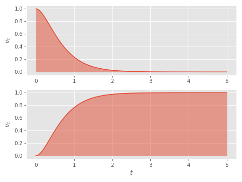
And when we talk about starting distance, we have the same problem as when we talk about stopping or starting time - at what point do we actually consider the start complete? We can't just take the integral to infinity any more because the distance travelled would be infinite too!
So we need to use the same solution as we did for stopping time. We need to first compute a starting time (defined as the time taken for the velocity to get within some threshold of the target), and then from this compute the distance travelled during that time.
For the distance travelled, we can compute the integral from \( 0 \) to the starting time \( t \) assuming initial velocity, and acceleration are zero \( v_0 = 0 \), \( a_0 = 0 \).
\begin{align*} d &= (\tfrac{-j_1}{y^2} \cdot e^{-y \cdot t} + \tfrac{-j_0 - j_1 \cdot t}{y} \cdot e^{-y \cdot t} + \tfrac{j_1}{y^2} + \tfrac{j_0}{y} + c \cdot t)\\ &- (\tfrac{-j_1}{y^2} \cdot e^{-y \cdot 0} + \tfrac{-j_0 - j_1 \cdot 0}{y} \cdot e^{-y \cdot 0} + \tfrac{j_1}{y^2} + \tfrac{j_0}{y} + c \cdot 0) \\ d &= (\tfrac{-j_1}{y^2} \cdot e^{-y \cdot t} + \tfrac{-j_0 - j_1 \cdot t}{y} \cdot e^{-y \cdot t} + \tfrac{j_1}{y^2} + \tfrac{j_0}{y} + c \cdot t) - (\tfrac{-j_1}{y^2} + \tfrac{-j_0}{y} + \tfrac{j_1}{y^2} + \tfrac{j_0}{y}) \\ d &= \tfrac{-(a_0 + (v_0 - c) \cdot y)}{y^2} \cdot e^{-y \cdot t} + \tfrac{-(v_0 - c) - (a_0 + (v_0 - c) \cdot y) \cdot t}{y} \cdot e^{-y \cdot t} + \tfrac{a_0 + (v_0 - c) \cdot y}{y^2} + \tfrac{v_0 - c}{y} + c \cdot t\\ d &= \tfrac{-(0 + (0 - c) \cdot y)}{y^2} \cdot e^{-y \cdot t} + \tfrac{-(0 - c) - (0 + (0 - c) \cdot y) \cdot t}{y} \cdot e^{-y \cdot t} + \tfrac{0 + (0 - c) \cdot y}{y^2} + \tfrac{0 - c}{y} + c \cdot t\\ d &= \tfrac{c}{y} \cdot e^{-y \cdot t} + \tfrac{c + (c \cdot y) \cdot t}{y} \cdot e^{-y \cdot t} + \tfrac{-c}{y} + \tfrac{-c}{y} + c \cdot t\\ d &= e^{-y \cdot t} \cdot \left(\tfrac{c}{y} + \tfrac{c + (c \cdot y) \cdot t}{y} \right) - \tfrac{2 \cdot c}{y} + c \cdot t\\ d &= e^{-y \cdot t} \cdot \left(\tfrac{2 \cdot c}{y} + c \cdot t \right) - \tfrac{2 \cdot c}{y} + c \cdot t\\ \end{align*}
In code it looks something like this:
def character_starting_distance(
    v_goal,   # Goal Velocity
    halflife, # Halflife
    v_eps     # Velocity Threshold
    ):

    y = halflife_to_damping(halflife) / 2.0

    t = character_starting_time(v_goal, halflife, v_eps)

    return np.exp(-y*t)*(2*v_goal/y + v_goal*t) - 2*v_goal/y + v_goal*t
This leaves us with one final problem. How can we compute the half-life from the starting distance. At a first glance it looks like it is going to be really tricky to re-arrange our previous equation in terms of \( y \) - but with a good substitution a nice solution pops out:
\begin{align*} z &= -(W(-\tfrac{\epsilon}{e}) + 1) \\ t &= -\tfrac{W(-\tfrac{\epsilon}{e}) + 1}{y} = \tfrac{z}{y} \end{align*}
then
\begin{align*} d &= e^{-y \cdot t} \cdot \left(\tfrac{2 \cdot c}{y} + c \cdot t \right) - \tfrac{2 \cdot c}{y} + c \cdot t\\ d &= e^{-z} \cdot \left(\tfrac{2 \cdot c}{y} + c \cdot \tfrac{z}{y} \right) - \tfrac{2 \cdot c}{y} + c \cdot \tfrac{z}{y}\\ d \cdot y &= e^{-z} \cdot (2 \cdot c + c \cdot z ) - 2 \cdot c + c \cdot z \\ y &= \frac{e^{-z} \cdot c \cdot (z + 2 ) + c \cdot (z - 2)}{d} \\ \end{align*}
Which in code can be implemented like this:
def character_halflife_from_starting_distance(
    v_goal,        # Goal Velocity
    d,             # Stopping Distance
    v_eps,         # Velocity Threshold
    ):

    v_scale = v_eps / v_goal
    z = -(lambertw(-v_scale / np.e, -1).real + 1)

    return damping_to_halflife(2*(np.exp(-z)*v_goal*(z + 2) + v_goal*(z - 2)) / d)
And with that we have all of the functions we need for estimating starting and stopping times and distances, as well their equivalents for fitting spring parameters.
True Half-Life
Doing all of this reminded me of something very dissatisfying about my original article on springs, which I can now fix or at least - suggest an improvement on.
When I introduced the concept of the half-life for spring dampers I defined it as follows (where \(0.69314718056 = ln(2) \)):
def halflife_to_damping(halflife, eps=1e-5):
    return (4.0 * 0.69314718056) / (halflife + eps)

def damping_to_halflife(damping, eps=1e-5):
    return (4.0 * 0.69314718056) / (damping + eps)
and I gave a very hand-wavy explanation about where this definition comes from.
The basic issue is that the concept of half-life doesn't really make sense when we talk about springs rather than simple dampers - because different initial spring velocities and targets will mean the time taken to get half-way to the target is not constant. And even worse, a spring can get half-way-there to the target but not be half-way-done, if it is going to over-shoot the target like we saw before.
But even so, if you measure how long it takes a character with initial velocity \( 1 \), initial acceleration \( 0 \), target velocity \( 0 \) and a half-life \( 0.5 \) to get half-way to the target you'll notice that it isn't at \( t = 0.5 \):
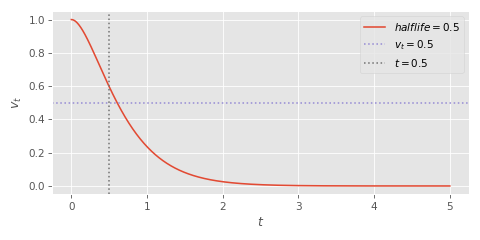
That's because the numbers I provided in that article really were fudged. The use of \( ln(2) \) gets us into the right ballpark, but ultimately they're just a good heuristic for roughly how long it takes to get half-way-there for the kind of the initial states you'd expect to encounter in real use.
But with our functions we've just derived we can compute the exact damping required for a critical spring with initial velocity \( 0 \) that travels half the distance to the target after \( 0.5 \) seconds:
\begin{align*} 2 \cdot -(W(\tfrac{-0.5}{e}) + 1) &= 3.356693980033321 \\ \end{align*}
The resulting value \( 3.356693980033321 \) is pretty close to our fudge \( 4.0 \cdot 0.69314718056 = 2.77258872224 \) from before. So the difference isn't massive. But if we wanted something with a little more concrete mathematical definition we could replace our equations from before with the new true half-life.
def true_halflife_to_damping(true_halflife, eps=1e-5):
    return 3.356693980033321 / (true_halflife + eps)

def damping_to_true_halflife(damping, eps=1e-5):
    return 3.356693980033321 / (damping + eps)

def halflife_to_true_halflife(halflife):
    return (halflife * 4.0 * 0.69314718056) / (3.356693980033321)

def true_halflife_to_halflife(true_halflife):
    return (true_halflife * 3.356693980033321) / (4.0 * 0.69314718056)
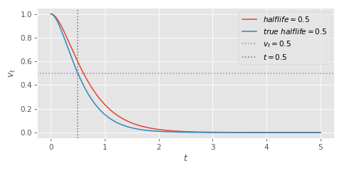
And here we can see the difference between the two when plotted.
Summary
Why is all of this useful? Well, not only are stopping and starting distances potentially more user-friendly than half-lives for configuring movement models, but this is another fantastic way to try and fit spring parameters from animation data.
If you can measure the stopping time and/or distance in your animation data it should be easy to compute the corresponding half-life. This you could potentially average over multiple starts and stops, or fit to different values in different contexts (e.g. walk vs run).
For example, we know that Usain Bolt can run 100m in 9.58 seconds. We also know that his max speed is 12.42m/s. That gives us an approximate half-life of either \( 1.96 \) for fit by distance distance or \( 1.73 \) for fit by time (with a threshold of 0.05m/s), which is not so far from our previous half-life of \( 1.90 \).
Appendix
After writing this I realised that there was a way to compute a stopping time which takes into account the initial acceleration. If we want to account for the fact that the spring might cross the x-axis we can split the computation into two. First: we can find the time at which the velocity reaches its peak and then add this time to the stopping time computed starting from that peak instead.
So first that means we need to compute the time of the peak velocity. This can be found as the time at which the derivative of our spring function (i.e. the acceleration) hits zero:
\begin{align*} a_t &= a_0 \cdot e^{-y \cdot t} - t \cdot j_1 \cdot y \cdot e^{-y \cdot t} \\ 0 &= a_0 \cdot e^{-y \cdot t} - t \cdot j_1 \cdot y \cdot e^{-y \cdot t} \\ 0 &= (a_0 - t \cdot j_1 \cdot y) \cdot e^{-y \cdot t} \\ 0 &= a_0 - t \cdot j_1 \cdot y \\ a_0 &= t \cdot j_1 \cdot y \\ t &= \tfrac{a_0}{j_1 \cdot y} \\ t &= \tfrac{a_0}{(a_0 + v_0 \cdot y) \cdot y} \\ t &= \tfrac{a_0}{a_0 \cdot y + v_0 \cdot y^2} \\ \end{align*}
Or in code:
def character_stopping_peak_velocity_time(
    v,        # Initial Velocity
    a,        # Initial Acceleration
    halflife, # Halflife
    ):

    y = halflife_to_damping(halflife) / 2.0

    return a / (a*y + v*y*y)
If this time is greater than zero, we need to compute the new spring velocity at that time and plug that into our previous stopping time function (which will work perfectly since we know the acceleration at this time is zero). But if this returns a time less than zero we still need to compute the stopping time taking into account the initial acceleration. This can be computed using the product logarithm but the derivation is a little more complex than before:
\begin{align*} v_t &= (v_0 - c) \cdot e^{-y \cdot t} + t \cdot (a_0 + (v_0 - c) \cdot y) * e^{-y \cdot t} + c \\ \epsilon &= (1 - 0) \cdot e^{-y \cdot t} + t \cdot (a_0 + (1 - 0) \cdot y) \cdot e^{-y \cdot t} + 0 \\ \epsilon &= e^{-y \cdot t} + t \cdot (a_0 + y) \cdot e^{-y \cdot t} \\ \epsilon &= (1 + t \cdot (a_0 + y)) \cdot e^{-y \cdot t} \\ -\epsilon &= (- t \cdot (a_0 + y) - 1) \cdot e^{-y \cdot t} \\ -e^{-y/(a_0 + y)} \cdot \epsilon &= (- t \cdot (a_0 + y)-1 ) \cdot e^{-y \cdot t - y/(a_0 + y)} \\ -e^{-y/(a_0 + y)} \cdot \epsilon \cdot y &= (- y \cdot t \cdot (a_0 + y)-y ) \cdot e^{-y \cdot t - y/(a_0 + y)} \\ -\frac{e^{-\frac{y}{a_0+y}} \cdot \epsilon \cdot y}{a_0 + y} &= (- y \cdot t - y/(a_0 + y)) \cdot e^{-y \cdot t - y/(a_0 + y)} \\ -y \cdot t - y/(a_0 + y) &= W \left( -\frac{e^{-y/(a_0 + y)} \cdot \epsilon \cdot y}{a_0 + y} \right) \\ t + \frac{1}{a_0 + y} &= \frac{-W \left( -\frac{e^{-y/(a_0 + y)} \cdot \epsilon \cdot y}{a_0 + y} \right)}{y} \\ t &= -\frac{W \left( -\frac{e^{-y/(a_0 + y)} \cdot \epsilon \cdot y}{a_0 + y} \right)}{y} - \frac{1}{a+y} \\ \end{align*}
Putting it all together in code it looks something like this:
def character_velocity(
    v,        # Initial Velocity
    a,        # Initial Acceleration
    c,        # Target Velocity
    halflife, # Halflife
    t         # Time Delta
    ):

    y = halflife_to_damping(halflife) / 2.0
    j0 = v - c
    j1 = a + j0*y

    return np.exp(-y*t)*(j0 + j1*t) + c

def character_stopping_time_approx(
    v,        # Initial Velocity
    halflife, # Halflife
    v_eps,    # Velocity Threshold
    ):

    y = halflife_to_damping(halflife) / 2.0

    v_scale = v_eps / v

    return -(lambertw(-v_scale / np.e, -1).real + 1) / y

def character_stopping_time(
    v,        # Initial Velocity
    a,        # Initial Acceleration
    halflife, # Halflife
    v_eps,    # Velocity Threshold
    ):

    y = halflife_to_damping(halflife) / 2.0

    t_p = character_stopping_peak_velocity_time(v, a, halflife)
    v_p = character_velocity(v, a, 0.0, halflife, t_p)

    v_scale = v_eps / v
    a_scale = a / v

    return np.where(t_p > 0.0,
        t_p + character_stopping_time_approx(abs(v_p), halflife, v_eps),
        -lambertw(-(np.exp(-y / (a_scale + y))*v_scale*y) /
            (a_scale + y), -1).real / y - (1 / (a_scale + y)))
Now we can compute the exact stopping time even when the initial acceleration is not zero.
However - I will note that I've found this computation to be pretty bad from a numerical stability standpoint - and it also requires the lambertw function to support sufficient input values of less than \( -\tfrac{1}{e} \) (which the above C++ implementation does not).
And here are all the functions from this post in one listing:
import numpy as np
from scipy.special import lambertw

def halflife_to_damping(halflife, eps=1e-5):
    return (4.0 * 0.69314718056) / (halflife + eps)

def damping_to_halflife(damping, eps=1e-5):
    return (4.0 * 0.69314718056) / (damping + eps)

def true_halflife_to_damping(true_halflife, eps=1e-5):
    return 3.356693980033321 / (true_halflife + eps)

def damping_to_true_halflife(damping, eps=1e-5):
    return 3.356693980033321 / (damping + eps)

def halflife_to_true_halflife(halflife):
    return (halflife * 4.0 * 0.69314718056) / (3.356693980033321)

def true_halflife_to_halflife(true_halflife):
    return (true_halflife * 3.356693980033321) / (4.0 * 0.69314718056)

####################

def character_position(
    x,        # Initial Position
    v,        # Initial Velocity
    a,        # Initial Acceleration
    c,        # Target Velocity
    halflife, # Halflife
    t         # Time Delta
    ):

    y = halflife_to_damping(halflife) / 2.0
    j0 = v - c
    j1 = a + j0*y

    return np.exp(-y*t)*(-j1/(y*y) + (-j0-j1*t)/y) + j1/(y*y) + j0/y + c*t + x

def character_velocity(
    v,        # Initial Velocity
    a,        # Initial Acceleration
    c,        # Target Velocity
    halflife, # Halflife
    t         # Time Delta
    ):

    y = halflife_to_damping(halflife) / 2.0
    j0 = v - c
    j1 = a + j0*y

    return np.exp(-y*t)*(j0 + j1*t) + c

def character_acceleration(
    v,        # Initial Velocity
    a,        # Initial Acceleration
    c,        # Target Velocity
    halflife, # Halflife
    t         # Time Delta
    ):

    y = halflife_to_damping(halflife) / 2.0
    j0 = v - c
    j1 = a + j0*y

    return np.exp(-y*t)*(a - j1*y*t)

####################

def character_stopping_inflection_time(
    v,        # Initial Velocity
    a,        # Initial Acceleration
    halflife, # Halflife
    ):

    y = halflife_to_damping(halflife) / 2.0

    return -v / (a + v*y)

def character_stopping_peak_velocity_time(
    v,        # Initial Velocity
    a,        # Initial Acceleration
    halflife, # Halflife
    ):

    y = halflife_to_damping(halflife) / 2.0

    return a / (a*y + v*y*y)

def character_stopping_distance_approx(
    v,        # Initial Velocity
    halflife, # Halflife
    ):

    y = halflife_to_damping(halflife) / 2.0

    return np.abs(2*v / y)

def character_stopping_distance(
    v,        # Initial Velocity
    a,        # Initial Acceleration
    halflife, # Halflife
    ):

    y = halflife_to_damping(halflife) / 2.0

    t = character_stopping_inflection_time(v, a, halflife)

    i0 = (v*y*2 + a) / (y * y)
    it = (np.exp(-y*t) / (y*y)) * (t*a*y + v*y*(t*y+2) + a)

    return np.where(t > 0.0, abs(i0 - it) + abs(it), abs(i0))

def character_stopping_time_approx(
    v,        # Initial Velocity
    halflife, # Halflife
    v_eps,    # Velocity Threshold
    ):

    y = halflife_to_damping(halflife) / 2.0

    v_scale = v_eps / v

    return -(lambertw(-v_scale / np.e, -1).real + 1) / y

def character_stopping_time(
    v,        # Initial Velocity
    a,        # Initial Acceleration
    halflife, # Halflife
    v_eps,    # Velocity Threshold
    ):

    y = halflife_to_damping(halflife) / 2.0

    t_p = character_stopping_peak_velocity_time(v, a, halflife)
    v_p = character_velocity(v, a, 0.0, halflife, t_p)

    v_scale = v_eps / v
    a_scale = a / v

    return np.where(t_p > 0.0,
        t_p + character_stopping_time_approx(abs(v_p), halflife, v_eps),
        -lambertw(-(np.exp(-y / (a_scale + y))*v_scale*y) /
            (a_scale + y), -1).real / y - (1 / (a_scale + y)))

def character_halflife_from_stopping_distance(
    v,        # Initial Velocity
    d,        # Distance
    ):

    return damping_to_halflife(4.0*v / d)

def character_halflife_from_stopping_time(
    v,        # Initial Velocity
    t,        # Stopping Time
    v_eps,    # Velocity Threshold
    ):

    v_scale = v_eps / v

    return damping_to_halflife(2.0 * -(lambertw(-v_scale / np.e, -1).real + 1) / t)

####################

def character_starting_time(
    v_goal,   # Goal Velocity
    halflife, # Halflife
    v_eps     # Velocity Threshold
    ):

    return character_stopping_time_approx(v_goal, halflife, v_eps)

def character_starting_distance(
    v_goal,   # Goal Velocity
    halflife, # Halflife
    v_eps     # Velocity Threshold
    ):

    y = halflife_to_damping(halflife) / 2.0

    t = character_starting_time(v_goal, halflife, v_eps)

    return abs(np.exp(-y*t)*(2*v_goal/y + v_goal*t) - 2*v_goal/y + v_goal*t)

def character_halflife_from_starting_time(
    v_goal,   # Goal Velocity
    t,        # Stopping Time
    v_eps,    # Velocity Threshold
    ):

    return character_halflife_from_stopping_time(v_goal, t, v_eps)

def character_halflife_from_starting_distance(
    v_goal,   # Goal Velocity
    d,        # Stopping Distance
    v_eps,    # Velocity Threshold
    ):

    v_scale = v_eps / v_goal
    z = -(lambertw(-v_scale / np.e, -1).real + 1)

    return damping_to_halflife(2*(np.exp(-z)*v_goal*(z + 2) + v_goal*(z - 2)) / d)