Filtering, Convolutions, and Quaternions
01/03/2025
In my previous article on Animation Quality I mentioned something a bit cryptic - which is that if you talk to signal processing folks, they'll tell you that almost everything we do in terms of handling the temporal aspect of animation data is wrong!
This topic came up again at work recently, and I thought I should finally do an article about exactly what I meant by this, and take a detailed look over another area of animation programming which I feel is probably a little neglected. So let's get into it.
Contents
- Gaussian Smoothing
- Weighted Sum
- Filtering and Convolution
- Convolution Composition
- Up-Sampling / Interpolation
- Down-Sampling / Summarization
- Velocities
- Key-framed Animation
- Frequency Analysis
- Summary
- Conclusion
Gaussian Smoothing
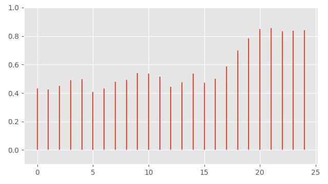
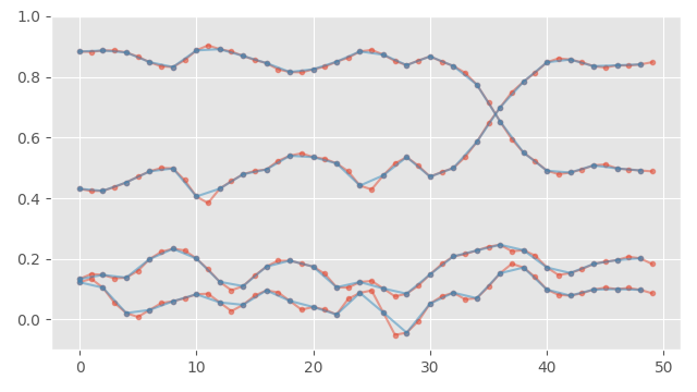
Let's start with a motivating example that involves a classic filter: given a time-series of rotation data, encoded as quaternions and unrolled:
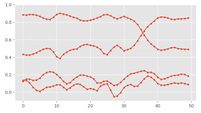
How would we go about smoothing this data?
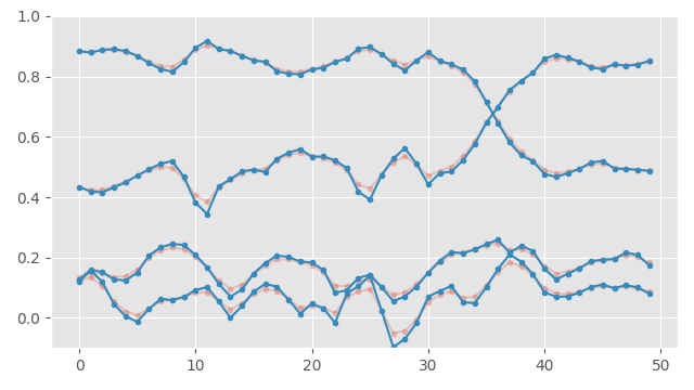
Well, here is one idea that might come to mind: we could apply a Gaussian smoothing filter to each component of the quaternion independently, and then re-normalize all of the quaternions at each frame. Sounds reasonable enough. Well, if we do that we end up with something like this:
Here you can see the smoothed version in blue. That looks pretty good... but what exactly have we done here?
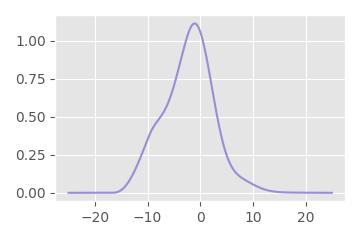
Well, the Gaussian filter is essentially, for each frame, performing a weighted sum (or averaging) over a small window of quaternion coefficients centered at that frame. The weights for this weighted sum (i.e. the kernel of the filter) are given by the Gaussian function, hence the name. Even though the Gaussian function technically goes on forever to the left and right, here I have cut it off at three times the width of the standard deviation, as it is pretty close to zero beyond this point:
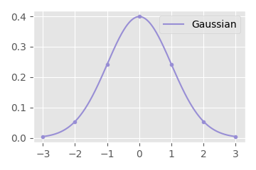
With this filter, the standard deviation of the Gaussian can be used to control the amount of smoothing applied.
Here is how we might implement the above Gaussian smoothing on the raw quaternion coefficients in C++:
// Gaussian function
float kernel_gaussian(float x, float std)
{
    return expf(-(x*x) / (2*std*std)) / (std*sqrtf(2*M_PI));
}

void quat_smooth_gaussian_raw(
    slice1d<quat> smoothed,         // Output smoothed rotations
    const slice1d<quat> rotations,  // Input rotations
    float std = 1.0f)               // Gaussian standard deviation
{
    int nframes = rotations.size;

    // Compute the window size needed to cover 3x the std
    int window = (int)ceilf(std * 3);

    // Loop over each frame
    for (int i = 0; i < nframes; i++)
    {
        // Temporary variable to accumulate weighted sum
        quat q = quat_zero();

        // Loop over all frames in the window
        for (int k = -window; k <= +window; k++)
        {
            // If the frame is within a valid range
            if (i + k >= 0 && i + k < nframes)
            {
                // Add rotation to accumulator, scaled by gaussian weight
                q = q + kernel_gaussian(k, std) * rotations(i + k);
            }
        }

        // Renormalize resulting quaternion
        smoothed(i) = quat_normalize(q);
    }
}
(Note: Given that kernel_gaussian is a function of only k and std, if we wanted we could avoid evaluating it many times in the innermost loop by pre-computing the function for all expected values of k.)
And here is a visualization of the kind of effect this smoothing produces if we apply it to some real animation data (slowed down a bit for demonstration):
So, is filtering quaternions really that simple? Just apply the filter to each component individually then renormalize?
Well if your quaternions are unrolled, fairly densely sampled, and do not contain any sudden discontinuities - yeah pretty much. That's going to work 99% of the time. But why?
Weighted Sum
The reason why, is that any kind of filter we apply, is basically going to come down to computing weighted sums of different groups of quaternions from the input signal. Quaternion weighted sums are something I've already talked fairly extensively in my article on quaternion weighted averages - and pretty much everything written there applies here too.
One thing I didn't cover in that article is what happens with negative weights. This is important for us because filters such as the classic (and incredibly confusingly named) "unsharp mask" (which is often used for sharpening images) often do have negative weights:
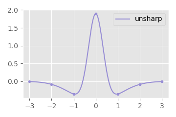
The method of weighted-sum I champion in my previous article is to compute the weighted sum of the outer-product of the quaternions and find the largest eigen vector of the resulting matrix. Luckily this method works perfectly well with negative weights. For example, here is the result of using the eigen-vector-based method with the unsharp mask kernel above, rather than doing the weighted sum in the raw quaternion space:
We can see it amplifies the changes in the signal exactly as expected. But averaging in the raw quaternion space works too (providing our signal is unrolled and densely sampled) - here is what that looks like on this example:
As you can see, the result is almost identical.
The only weighted-sum method we need to be careful with is if we want to do things in the log space. The problem is that the log space cannot be (entirely) "unrolled" - so unlike the raw quaternion space, discontinuities are unavoidable. We therefore need to do what I describe in the appendix of my article on quaternion weighted averages: make the rotations in the weighted sum "relative" to something meaningful before we average them. While it's possible to choose any appropriate rotation (e.g. the bind pose can be an option just as before) - a nice choice is the central quaternion in the window.
In code it looks something like this:
void quat_smooth_gaussian_log(
    slice1d<quat> smoothed,         // Output smoothed rotations
    const slice1d<quat> rotations,  // Input rotations
    float std = 1.0f)               // Gaussian standard deviation
{
    int nframes = rotations.size;

    // Compute the window size needed to cover 3x the std
    int window = (int)ceilf(std * 3);

    // Loop over each frame
    for (int i = 0; i < nframes; i++)
    {
        // Temporary variables to accumulate log-rotation and weight sum
        vec3 v = vec3();
        float w = 0.0;

        // Reference rotation from the center of the window
        quat r = rotations(i);

        // Loop over all frames in the window
        for (int k = -window; k <= +window; k++)
        {
            // If the frame is within a valid range
            if (i + k >= 0 && i + k < nframes)
            {
                // Compute kernel weight
                float kw = kernel_gaussian(k, std);

                // Add scaled log-rotation and weight to accumulators
                v = v + kw * quat_log(quat_inv_mul(r, rotations(i + k)));
                w = w + kw;
            }
        }

        // Take out of exponential map and multiply back reference rotation
        smoothed(i) = quat_mul(r, quat_exp(v / w));
    }
}
Since we are no longer doing quaternion re-normalization, we now need to also accumulate our own sum of the kernel weights, and use this to re-normalize before we convert back using the exponential map.
This same method is presented in a lot more depth in this over-20-year-old paper. This log-based method where we choose the central quaternion in the window can be seen as the equivalent of doing a slerp instead of a nlerp.
This is what the log-space method looks like on our previous signal. The difference is again really minimal compared to doing things in the raw quaterion space:

So that is basically it: filtering quaternions requires doing weighted sums, and the options for doing that are pretty much the same as when we do a weighted average. Either use the eigen-vector-based method, or make sure your quaternions are unrolled and apply the filter in the raw quaternion space and re-normalize, or if you are feeling fancy, use the relative-rotation-log-space method presented above.
But why did I bring this up in the first place, and why did I say that the way we tend to do things in animation is wrong? Well, perhaps more accurate is that the way we think about the temporal aspect of animation data is often wrong...
Filtering and Convolution
When we think about filtering, we might think of it as a kind of discrete process like the one visualized above, where we have a kernel of a given "window size", which we slide element by element over an array.
However, it can be very powerful to think more abstractly about this process, and consider the continuous generalization of this, where we have one continuous function which "slides" over another continuous function, and we compute the integral (the continuous equivalence of the weight sum) at every point. This is of course Convolution.
But how can we represent motion capture data as a continuous function? One way is to think of our animation data as a special kind of continuous function, made up of a series of so called "Dirac delta functions" located at our data-points, with undefined values everywhere else:
For motion capture data at least, I think this is a more accurate way to think about things than the connect-the-dot plots we're used to. That's because our motion capture data is indeed a series of snapshots of the state of the world - what happened in-between those snapshots we don't actually know.
Given a signal like this, when we slide (for example) our Gaussian kernel over it, we are still going to recover the same discrete weighted sum as before (assuming we disregard undefined values), except that the "output" of the filter is now defined everywhere, not just at the discrete locations where we had our samples:
I like to think of our arrays of values as a kind of sparse representation of these continuous functions which are made up of a series of Diracs. And when we do discrete filtering on these arrays, we can think of this just as a kind of optimization of the convolution process where we are working efficiently on this internal representation directly.
I think under this view it becomes clear that we don't need to consider something like a Gaussian filter as just a kind of discrete process that takes an array of values as input, and array of kernel values, and produces an of values as array as output.
Instead we can consider smoothing our data by a Gaussian filter as a convolution which takes a continuous signal as input (represented as a sparse array of data-points), and outputs a continuous signal, which we are then going to sample at regularly spaced intervals and encode back again as a sparse array of data-points.
This is important when we come back to think about down-sampling and up-sampling of animation data.
Convolution Composition
So why is it good to think about things in terms continuous convolutions? I think there are two reasons.
The first reason is something I think game developers often under-estimate: simply that a large number of very smart people have spent a long time thinking about things like convolutions. If there is some kind of problem you want to solve - if you are able to frame it in terms of convolutions - there is a good chance someone already came up with an answer.
For example, many people have already derived a huge number of filters for all sorts of purposes which we can take inspiration from.
The second reason, which goes hand-in-hand with the first, is that (like matrices) convolutions are easy and efficient to compose.
We know that when you have two matrices \( \mathbf{A} \), and \( \mathbf{B} \), and you want to transform a bunch of vectors by \( \mathbf{B} \), and then by \( \mathbf{A} \), you can pre-multiply \( \mathbf{C} = \mathbf{A}\ \mathbf{B} \) to get a new matrix \( \mathbf{C} \) which you can then multiply all of your vectors by to perform the same thing. This can potentially save huge amounts of computation.
Convolutions are exactly the same! If you have a signal you want to convolve by a filter \( \mathbf{B} \), and then by a filter \( \mathbf{A} \), you can instead convolve the filter \( \mathbf{B} \) by \( \mathbf{A} \) to get a new filter \( \mathbf{C} \), \( \mathbf{C} = \mathbf{A} * \mathbf{B} \), which you then convolve your original signal by. This is equally powerful! Instead of performing a bunch of convolutions in sequence, we can compute a filter which will perform all of them for us at once!
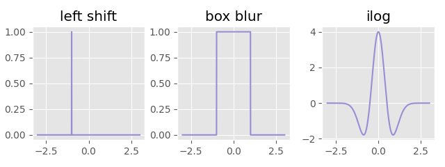
For example, if we take our two different kernel functions from before:
We can apply these filters one by one and get the following:
(Note: the mathematical definition of convolution mirrors the sliding kernel on the Y-axis, we just haven't encountered that yet because all of our kernels have been symmetric before this.)
Or, we can convolve the filters together to get the following:
And convolve our signal with this to get exactly the same result:
Understanding the algebra and mathematical framework around convolutions can be a very powerful tool for all kinds of signal processing tasks and give us a deeper understanding of the underlying process, which in turn can help inform the technical decisions we make.
Up-Sampling / Interpolation
We might like to think about up-sampling as a kind of discrete process where we (for example) double the resolution of a signal, but the more general way to think about up-sampling is as "filling in the gaps" of a sparsely sampled signal: given some arbitrary location (or locations) on the x-axis we can consider up-sampling as wanting to estimate the best possible guess for what the true original signal value was at that point.
There are many different approaches to interpolation. Most likely you are already familiar with linear interpolation, and might well have tried others such as spline interpolation, or maybe even something like radial basis functions, but as it turns out, for many kinds of interpolation, there is often a convolutional kernel which defines it.
For example, linear interpolation is equivalent to convolving our signal with the "tent" kernel:
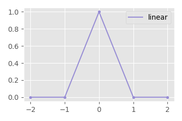
This performs a kind of cross-fade between the values, producing our familiar connect-the-dots plot. On quaternions this will be equivalent to a nlerp when performed in the raw quaternion space, and equivalent to a slerp when performed in the relative log space:
If we use other kernels, we can get other results - and there are many kernels that have been well studied and proven to have nice properties of interpolation and up-sampling. For example, if we convolve with this kernel:
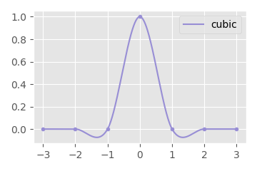
Given by the following equation:
\begin{align*} y &= \begin{cases} \phantom{-}\tfrac{3}{2}\ |x|^3 - \tfrac{5}{2}\ |x|^2 + 1\hspace{1.15cm}\ \text{if}\ \phantom{0 \lt} |x| \lt 1 \\ -\tfrac{1}{2}\ |x|^3 + \tfrac{5}{2}\ |x|^2 - 4\ |x| + 2\ \text{if}\ 1 \le |x| \le 2 \\ 0\hspace{4.1cm} \text{otherwise} \end{cases} \end{align*}
We get an almost identical result to the quaternion cubic interpolation method I talked about in an earlier article. This is the catmull-rom cubic interpolation kernel.
Here is how we might write the equivalent interpolation function in C++:
// Catmull-Rom cubic kernel function
float kernel_cubic(float x)
{
    x = fabsf(x);
    return
        x <= 1 ? (3.0f/2.0f)*x*x*x - (5.0f/2.0f)*x*x + 1 :
        (x > 1) && (x < 2) ? -(1.0f/2.0f)*x*x*x + (5.0f/2.0f)*x*x - 4*x + 2 : 0.0f;
}

quat quat_signal_interpolate_cubic_log(
    const slice1d<quat> rotations, float time, float dt)
{
    // Clamp time to valid range
    time = clampf(time, 0.0f, (rotations.size - 1) * dt);

    // Get the nearest frame for the given time
    int i = clamp((int)(time / dt), 0, rotations.size - 1);

    // Accumulated kernel weight
    float w = 0.0;

    // Accumulated output rotation
    vec3 r = vec3();

    // Cubic Kernel Width
    int kwidth = 2;

    // Loop over all nearby frames within the kernel width
    for (int k = -kwidth + 1; k <= kwidth; k++)
    {
        // If there is a valid sample at that frame
        if (i + k >= 0 && i + k < rotations.size)
        {
            // Sample the weight from the kernel function
            float kw = kernel_cubic(time / dt - i - k);

            // Accumulate the log-space relative rotation and weight
            r += kw * quat_log(quat_inv_mul(rotations(i), rotations(i + k)));
            w += kw;
        }
    }

    // Convert back from the log space
    return quat_mul(rotations(i), quat_exp(r / w));
}
There are other cubic interpolation schemes too given by other kernels. For example, here is a cubic kernel which looks at a window of three-frames either side of the center and has a nice smooth shape:
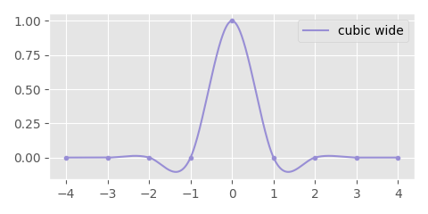
It's given by the following equation:
\begin{align*} y = \begin{cases} \phantom{-}\ \tfrac{4}{3}\ |x|^3 - \tfrac{7}{3}\ |x|^2 + 1 \hspace{1.4cm} \text{if}\ 0 \le |x| \lt 1 \\ -\tfrac{7}{12}\ |x|^3 + 3\ |x|^2 - \tfrac{59}{12}\ |x| + \tfrac{5}{2}\ \text{if}\ 1 \le |x| \lt 2 \\ \phantom{-}\tfrac{1}{12}\ |x|^3 - \tfrac{2}{3}\ |x|^2 +\ \tfrac{7}{4}\ |x| - \tfrac{3}{2}\ \text{if}\ 2 \le |x| \le 3 \\ 0\hspace{4.5cm} \text{otherwise} \end{cases} \end{align*}
And here is what this one looks like as used for interpolation:
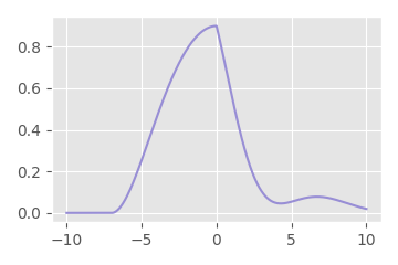
Naturally there is a huge variety of kernels that can be used for interpolation, each providing their own different flavor. But is there a theoretically "best" interpolation kernel? Kind of... the theoretically optimal interpolation is the sinc kernel:
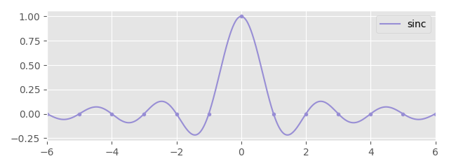
Given by the following function:
\begin{align*} \text{sinc}(x) = \frac{\sin(\pi x)}{\pi x} \end{align*}
This kernel in theory computes a perfect reconstruction of the original signal, assuming the signal was captured at a high enough sample rate.
Here is the result we get convolving with this kernel:
I think this is one of those magic moments in mathematics where you see something that hints at something much deeper... because to me at least, it is not at all immediately intuitive as to why convolving with this weird function should produce an optimal interpolation of the data.
But even if this kernel may be theoretically ideal, it has two practical issues. First, unlike the cubic kernels this function goes outwards for infinity, so we need to choose an appropriate cutting-off point. Unfortunately this is not easy as it does not decay very fast toward zero (like our Gaussian function for example).
Second, this is only theoretically optimal for input signals of infinite length and sufficient sampling frequency. Applying it to signals of a fixed length or those which are under-sampled can cause bad "edge-effects" at the fringes of the signal, or ringing when the signal is not sampled at a high enough rate:
A practical solution to these two issues is to multiply the \( sinc \) function by some kind of fixed-falloff window. For this there are a whole family of windowed \( sinc \) kernels.
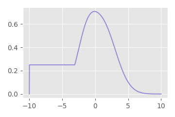
A popular choice from these is the lanczos kernel. Which windows the \( sinc \) function with another \( sinc \) function:
\begin{align*} \text{lanczos}(x, a) = \begin{cases} \text{sinc}(x)\ \text{sinc}(\tfrac{x}{a})\ \text{if} -a \lt x \lt a \\ 0 \hspace{2.3cm} \text{otherwise} \end{cases} \end{align*}
In this case the \( a \) parameter controls the width of the kernel. Here is a plot where \( a = 3 \) (a.k.a lanczos3).
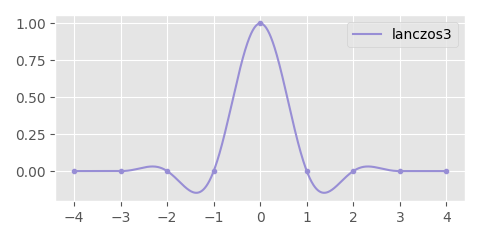
Here is the result we get with a lanczos3 kernel:
And here is how we might do lanczos interpolation in C++:
float sincf(float x)
{
    return fabsf(x) < 1e-8f ? 1.0f : sinf(M_PI * x) / (M_PI * x);
}

float kernel_lanczos(float x, int a)
{
    return x > -a && x < a ? sincf(x / a) * sincf(x) : 0.0f;
}

quat quat_signal_interpolate_lanczos_log(
    const slice1d<quat> rotations, float time, float dt, int kwidth)
{
    // Clamp time to valid range
    time = clampf(time, 0.0f, (rotations.size - 1) * dt);

    // Get the nearest frame for the given time
    int i = clamp((int)(time / dt), 0, rotations.size - 1);

    // Accumulated kernel weight
    float w = 0.0;

    // Accumulated output rotation
    vec3 r = vec3();

    // Loop over all nearby frames within the kernel width
    for (int k = -kwidth + 1; k <= kwidth; k++)
    {
        // If there is a valid sample at that frame
        if (i + k >= 0 && i + k < rotations.size)
        {
            // Sample the weight from the kernel function
            float kw = kernel_lanczos(time / dt - i - k, kwidth);

            // Accumulate the log-space relative rotation and weight
            r += kw * quat_log(quat_inv_mul(rotations(i), rotations(i + k)));
            w += kw;
        }
    }

    // Convert back from the log space
    return quat_mul(rotations(i), quat_exp(r / w));
}
In this code, all we've really changed from the cubic interpolation is the kernel function and the kernel width.
The windowed \( sinc \) kernels like lanczos give us a kind of control for performance vs theoretical backing. If we have a long, densely sampled signal, and can pay for the performance cost, we can choose a larger value for \( a \) to get a "better" interpolation. If we have a shorter, less densely sampled signal, or we can't pay the performance cost, we can choose a smaller value for \( a \) to minimize artefacts around abrupt changes and the edges of the animation, or make things as fast as possible.
Down-sampling / Summarization
Now that we've discussed up-sampling, what about down-sampling?
Let's start by looking at the ways people tend to down-sample animation data currently. There are two main methods I've seen used, and both have problems.
The first method I sometimes see used, is to take an average of pairs of frames, to reduce the resolution of the signal by half (e.g. from 60Hz to 30Hz). For example, this is often the default way things are done in many Machine Learning "pooling" operators. If we just plot the result of doing this, it doesn't take much to see why this might be a bad idea:
This effectively shifts the signal left by half a frame. That's because we are computing an average at sample locations that are not in the same locations as our original data-points. I wont go into too much detail here because I don't think I can explain the issue better than Bart Wronski's fantastic article on the subject.
You might think that a half-a-frame offset is not a big deal. In which case, I wish you the best of luck debugging off-by-a-half-frame errors if you ever need to do anything that involves syncing audio, video, and motion capture.
The second, more common method I see is to just take every other frame in the data again, to reduce the resolution by half:
This is far better, but still subtly wrong from a single processing perspective. This is equivalent to doing a nearest-neighbor down-sampling - which can create bad aliasing. This is an effect I'm sure you've seen when down-sampling images:
The effect might be less noticeable for animation data which typically contains a lot fewer high frequency details, but it is still there.
To avoid aliasing, before we down-sample, we need to first remove any frequencies which are too high to be represented in the down-sampled signal. The easiest way to do this is to process our signal using a filter with a width that matches the down-sampled sample rate we are targeting.
In this way we can think about up-sampling and down-sampling as like two sides of the same coin. The only difference is that when we down-sample we are going to scale our filter based on the desired sample interval to make it wider and flatter. For example, if we want to do a linear down-sampling by a factor of two, it means we should convolve with a double-width tent kernel, scaled down by a half, and then take samples from the resulting signal at the desired rate.
Another advantage of thinking about things in this way is that it becomes clear how to best down-sample at intervals which are not multiples of the original signal sample-rate...
Just like up-sampling, the result we get will depend on the kernel we choose. For example, here is the wide cubic kernel from before:
And again, just like before, the \( sinc \) filter is the theoretically optimal filter for this task. Here is an example of down-sampling using the \( sinc \) kernel:
But while it might be theoretically optimal, just like before there are practical issues to using this kernel. Again, the windowed \( sinc \) kernels allow us to decide on our preferred balance between performance and quality. And while larger values of \( a \) might be more effective at removing aliasing, they will also introduce over-shooting when the down-sampled frequency is too low.
So if up-sampling is akin to interpolation, then what is down-sampling akin to?
I like to think about down-sampling as "summarizing" a signal. Imagine opening your eyes (or a camera shutter) for just a second and observing a person moving. If you were asked to summarize what you had seen as a single pose/snapshot, how would you do it?
Well you could summarize it using the pose you saw right at center of the window of time. This would be equivalent to a nearest-neighbor style of down-sampling. But I think it's clear this gives a very biased impression of what you saw - if the person was moving very fast and changing their pose a lot then a minor difference in time might mean you give a very different answer. That would mean aliasing.
Instead it feels more fair to summarize that pose as some kind of weighted average of all the poses you saw over that short window of time. This is exactly what our convolution is doing in this down-sampling process - and the weights of that average across the window are exactly given by our kernel: the linear tent kernel gives a higher weight to the central pose but still takes into account the poses each side, and if we follow the mathematics we are eventually going to end up with the \( sinc \) giving the optimal way of summarizing a signal for a given sample rate.
But if down-sampling is "summarizing" the poses in a signal, then it matters how we are playing that signal back. For example, if we are down-sampling a signal to match our display device sample rate, or to increase playback speed of the animation then yes - the summarizing concept absolutely makes sense because each frame what we are going to display is meant to portray a kind of summarize of multiple frames in one "snapshot".
But if we are down-sampling to below our display device playback rate, just to reduce memory, with the intention of up-sampling or interpolating the result before we display it, then there isn't any need to summarize the signal beyond the device playback rate.
In this case, we can do something more clever. In fact, Bart Wronski convers this too in another fantastic blog post. We can compute an optimal down-sampling, such that when we up-sample by whichever kernel we intend to use, to whatever our desired playback rate is, we reconstruct something as similar as possible to the original signal.
I think the easiest way to actually set this up is using PyTorch's auto-differentiation. Here if we have a variable Xrot of shape [nframes, nbones, 4] representing some local joint rotations, we can optimize for the best down-sampling, assuming a linear up-sampling, in just a few lines of PyTorch.
dt = 1.0 / 60.0                     # Delta time
ssample = 4                         # Ratio by which to subsample
duration = dt * (len(Xrot) - 1)     # Total clip duration

# Linear interpolation kernel
def linear_kernel(x):
    return 1.0 - abs(torch.clip(x, -1, 1))

# Function for up-sampling via linear interpolation
def quat_upsample_linear(qs, t, qdt):
    i0 = torch.clip((t / qdt).long() + 0, 0, len(qs) - 1)
    i1 = torch.clip((t / qdt).long() + 1, 0, len(qs) - 1)
    w0 = linear_kernel(i0 - t / qdt)[:,None,None]
    w1 = linear_kernel(i1 - t / qdt)[:,None,None]
    return tquat.normalize(w0 * qs[i0] + w1 * qs[i1])

# Create initial guess at best sub-sampled version of the data
Xrot_ss = torch.tensor(Xrot[::ssample].copy(), dtype=torch.float32, requires_grad=True)

# Times at which to compute the interpolation for comparison (sampled at 600 Hz)
T = torch.linspace(0, duration, int(duration * 600))

# Create the target values using the ground truth
with torch.no_grad():
    Xrot_targ = quat_upsample_linear(torch.as_tensor(Xrot, dtype=torch.float32), T, dt)

# Run optimization
optim = torch.optim.SGD([Xrot_ss], lr=1.0)

for i in range(100):
    optim.zero_grad()

    Xrot_pred = quat_upsample_linear(tquat.normalize(Xrot_ss), T, ssample * dt)

    loss = torch.mean(torch.square(100.0 * (Xrot_targ - Xrot_pred)))
    loss.backward()

    print('%04i Loss: %f' % (i, loss.item()))

    optim.step()
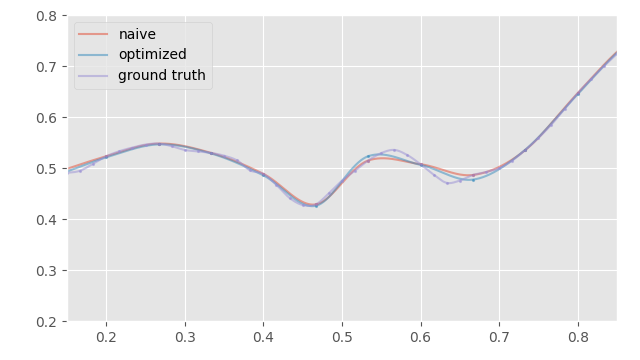
Here is an example of what this produces:
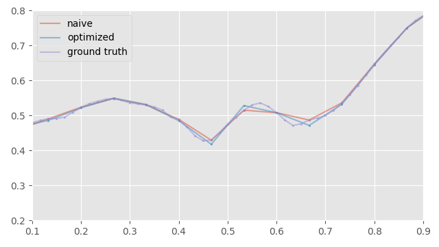
You can see that compared to the initial sub-sampling where I just take every other frame, this method distributes the errors more evenly across the samples. Here is a plot of those errors:
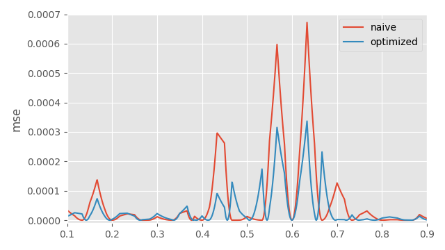
As expected, sub-sampling every frame produces zero error every other frame, but higher error in-between. Here is the result I get doing the same thing but assuming a cubic interpolation for up-sampling:
And here is a plot of the errors again:
One nice thing we can do with auto-differentiation is use more complex loss functions. For example, we might want to add in a forward-kinematics loss to account for error propagation down the chain:
Xrot_ss = torch.tensor(Xrot[::ssample].copy(), dtype=torch.float32, requires_grad=True)
Xpos_ss = torch.tensor(Xpos[::ssample].copy(), dtype=torch.float32)

T = torch.linspace(0, duration, int(duration * 600))

with torch.no_grad():
    Xpos_pred = upsample_cubic(Xpos_ss, T, ssample * dt)
    Xrot_targ = quat_upsample_cubic(torch.as_tensor(Xrot, dtype=torch.float32), T, dt)
    Xpos_targ = upsample_cubic(torch.as_tensor(Xpos, dtype=torch.float32), T, dt)
    _, Xglo_pos_targ = tquat.fk(Xrot_targ, Xpos_targ, parents)

optim = torch.optim.SGD([Xrot_ss], lr=0.001)

for i in range(100):
    optim.zero_grad()

    Xrot_pred = quat_upsample_cubic(tquat.normalize(Xrot_ss), T, ssample * dt)
    _, Xglo_pos_pred = tquat.fk(Xrot_pred, Xpos_pred, parents)

    loss_loc = torch.mean(torch.square(50.0 * (Xrot_targ - Xrot_pred)))
    loss_glo = torch.mean(torch.square(2.0 * (Xglo_pos_pred - Xglo_pos_targ)))
    loss = (loss_loc + loss_glo) / 2
    loss.backward()

    print('%04i Loss: %f, %f %f' % (i, loss.item(), loss_loc.item(), loss_glo.item()))

    optim.step()
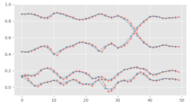
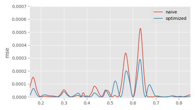
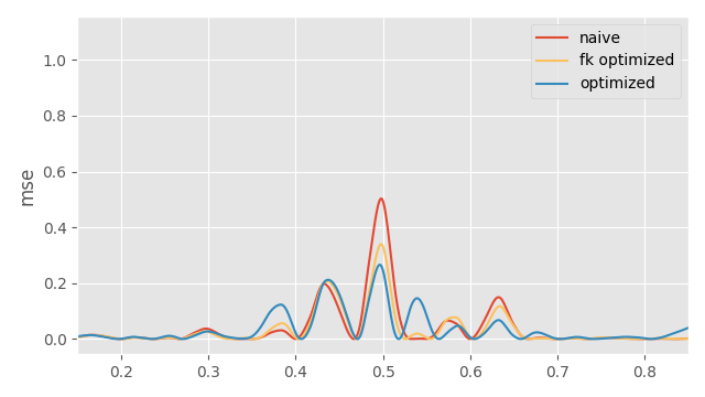
Here is a comparison plot for the global hand location in the final optimized result.
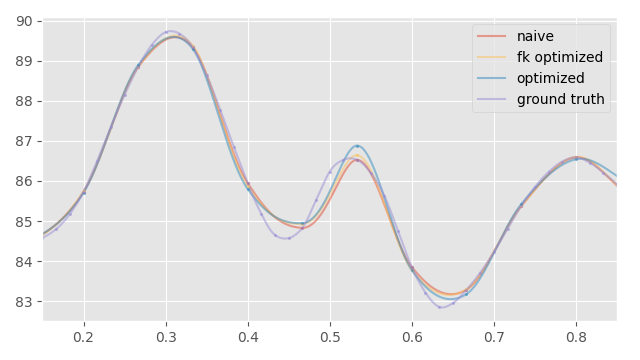
We can see that running the optimization in the local rotation space actually produces some over and under shooting on the global joint positions you get from the forward kinematics. Optimizing with the FK loss avoids these nicely. Here is a plot of the error in the world space for the hand:
To summarize: consider what the purpose of your down-sampling is. If you are adjusting playback speed, and/or down-sampling a signal to your desired playback rate, consider using a proper kernel over a nearest-neighbor approach to avoid aliasing.
If you are down-sampling for memory-savings, and/or have some particular up-sampling method in mind which you are going to use when playing back the animation, consider if you can optimize for the best possible down-sampling that might produce as close as possible to the interpolated result you want.
Velocities
Velocities are a key part of dealing with animation data. In a previous article I argued for the importance of treating velocities as first class citizens in animation systems. But to do this we require the ability to sample velocities directly from the animation data.
In that article, as well as my previous article on cubic interpolation of quaternions, I computed the velocity using the analytical derivative of the interpolation function. While this works nicely for linear and cubic interpolation, unfortunately it doesn't work in the general case.
For example, here is how I might compute the analytical derivative of a lanczos interpolation, and use it to output the velocity of the interpolation:
// sinc function derivative
float sincfdx(float x)
{
    return fabsf(x) < 1e-8f ? 0.0f :
        (M_PI * ((M_PI * x) * cosf(M_PI * x) - sinf(M_PI * x))) / squaref(M_PI * x);
}

// lanczos kernel derivative
float kernel_lanczosdx(float x, int a)
{
    return x > -a && x < a ?
        sincf(x / a) * sincfdx(x) + sincf(x) * (sincfdx(x / a) / a) : 0.0f;
}

void quat_signal_interpolate_lanczos_log_dx(
    quat& out_rot,
    vec3& out_ang,
    const slice1d<quat> rotations,
    float time, float dt, int kwidth)
{
    // Clamp time to valid range
    time = clampf(time, 0.0f, (rotations.size - 1) * dt);

    // Get the nearest frame for the given time
    int i = clamp((int)(time / dt), 0, rotations.size - 1);

    // Accumulated kernel weight
    float w = 0.0;
    float wdx = 0.0f;

    // Accumulated output rotation and angular velocity
    vec3 r = vec3();
    vec3 a = vec3();

    // Loop over all nearby frames within the kernel width
    for (int k = -kwidth + 1; k <= kwidth; k++)
    {
        // If there is a valid sample at that frame
        if (i + k >= 0 && i + k < rotations.size)
        {
            // Sample the weight and derivative from the kernel function
            float kw = kernel_lanczos(time / dt - i - k, kwidth);
            float kwdx = kernel_lanczosdx(time / dt - i - k, kwidth);

            // Compute relative log-space rotation
            vec3 lrot = quat_log(quat_inv_mul(rotations(i), rotations(i + k)));

            // Accumulate rotations, velocities, and weights
            r += kw * lrot;
            a += kwdx * lrot;
            w += kw;
            wdx += kwdx;
        }
    }

    // Convert back from the log space, accounting in velocity for normalization
    out_rot = quat_mul(rotations(i), quat_exp(r / w));
    out_ang = quat_mul_vec3(rotations(i), (w * a - r * wdx) / (dt * squaref(w)));
}
Surprisingly, doing this produces velocities which have a lot of tiny oscillations. We can see this if we compare it to the cubic interpolation method from the previous article:
This isn't due to some weird mathematics in the analytical derivative - if we compute the gradient via finite difference we will get exactly the same thing. So this is a real effect in the interpolated result - it's just that it is too small to really see on the pose itself.
And this effect is also not limited to just this kernel or this situation. It will occur to some extent in any case where the weights of the kernel require re-normalization. This means this always happens when (for example) down-sampling with a kernel width which is a non-integer multiple of the sample rate, no matter which kernel we use.
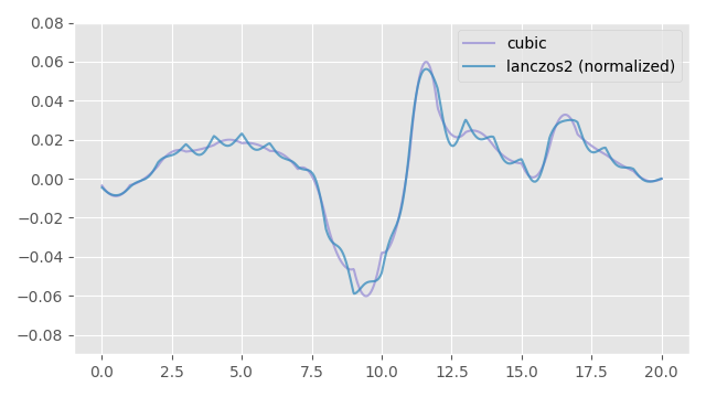
But why? Well, here is the result of interpolating a signal using a lanczos2 filter without re-normalizing the weights:
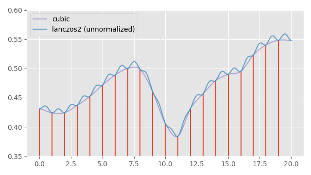
As you can see, when the kernel is not aligned with the data-points exactly, we get little bumps. This is because the weights of the lanczos2 kernel will sum to a value greater than one when it is not lined up exactly with the data-points. This causes a small bump, which will be larger the further way from zero our signal is.
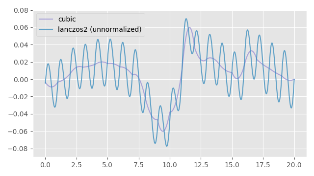
And here is the gradient of the above curve. These little bumps/oscillations are super amplified when we look at the gradient:
If we re-normalize the weights as we interpolate, the bumps in the output signal seem to disappear:
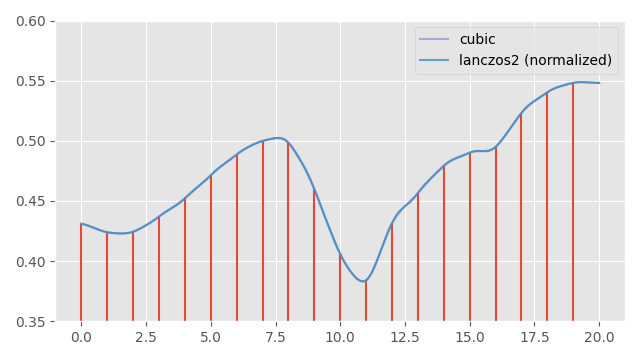
However, if we again look at the gradient, we can see that this re-normalization has not actually entirely fixed things here, and there are still some oscillations. These small oscillations are exactly the oscillations we are seeing in our visualization of animation velocities from above.
The basic issue is that (while it might have worked for our cubic interpolation) the instantaneous derivative of the filtering function is not guaranteed to be smooth or well behaved in the general case - and often is not - even when the output itself might look okay. So this approach of taking the derivative of the output and using that as the velocity wont work.
So what's the alternative?
Well, a much more robust approach to the handling of velocities is to compute the velocities in the input signal, and then filter those velocities just as we would the signal itself.
For example, we can compute velocity samples in the input signal via finite difference, and place these samples at the mid-points between our data samples:
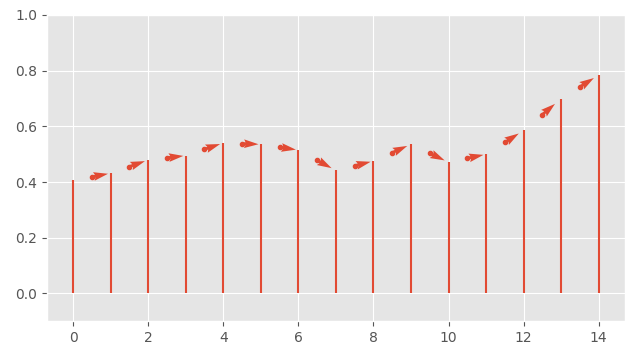
We can then filter these velocity samples by applying exactly the same filter we are using for our original samples - computing a weighted-sum of velocities in exactly the same way:
Here is how we might implement that in C++:
vec3 quat_signal_interpolate_velocity_lanczos(
    const slice1d<quat> rotations, float time, float dt, int kwidth)
{
    // Clamp time to valid range
    time = clampf(time, 0.0f, (rotations.size - 1) * dt);

    // Get the nearest frame for the given time
    int i = clamp((int)(time / dt), 0, rotations.size - 1);

    // Accumulated kernel weight
    float w = 0.0;

    // Accumulated output velocity
    vec3 a = vec3();

    // Loop over all nearby frames within the kernel width
    for (int k = -kwidth; k <= kwidth; k++)
    {
        // If there is a valid sample at that frame
        if (i + k + 0 >= 0 && i + k + 0 < rotations.size &&
            i + k + 1 >= 0 && i + k + 1 < rotations.size)
        {
            // Sample the weight from the kernel function
            float kw = kernel_lanczos(time / dt - i - k - 0.5f, kwidth);

            // Sample velocity via finite difference
            vec3 ka = quat_to_scaled_angle_axis(quat_abs(
                quat_mul_inv(rotations(i + k + 1), rotations(i + k + 0)))) / dt;

            // Accumulate angular velocity and weight
            a += kw * ka;
            w += kw;
        }
    }

    // Normalize and output
    return a / w;
}
It's important to remember that the velocity you get out here will not be the actual true velocity of the filtered output signal.
In most cases, however, this is actually a good thing - because as we just saw, the true velocity of the filtered output signal may not actually be very well behaved all. This filtered velocity, on the other hand, should always be smooth and artefact free.
This difference is most obvious if we filter data with a linear kernel, as doing so will still produce a smoothly varying velocity, which is obviously not the same as the real gradient of the interpolated signal itself, which we would expect to contain sudden jumps as we switch between data points:
And here is the same thing but shown on the character:
So to handle velocities in a general way we need to abandon the idea of using the analytical derivative of our interpolation function and instead filter the velocity of the input signal. This can be done generically by computing velocity samples by finite difference, and locating those velocity samples at the midpoints between the original data samples.
Key-framed Animation
The elephant in the room this whole article is the fact that key-framed animation data is not at all like motion capture data. It's not a series of snapshots where we don't know what happened in-between and we need to "guess" at the best interpolation. Most often, key-framed animation is represented by a series of curves, which means the animator has defined precisely how it should be interpolated and what the pose should be for any given arbitrary time in-between.
So how can we unify this world view with everything I've said above? Well... time to get into the weeds a bit and say some things I am certain a few people will disagree with.
Let's start with the easy case. If you have some lovingly made, key-framed animation data which is synced up with the display rate such that you know exactly what pose should be displayed on each frame - I would say don't mess with it. So if you are dealing with animated films, VFX, and anything else rendered offline, where this is most likely the case, feel free to disregard this whole article.
However, in video games, this is also very often not the case. Most often in video games the variable frame-rate means that our frames of animation are generally not in sync with the display, and instead we are almost always interpolating animation data on-the-fly to produce a pose at an arbitrary time. This is often the case even for canned animations and cinematics.
And this is kind of the crux of it, because at soon as we are performing some kind of interpolation of the key-framed animation, we need to accept that the poses the animator creates are just not the exact poses that are going to get presented on the screen. And, I would argue that on average you will get poses which more closely resemble the vision of the animator if you adopt a signal processing world view as outlined in this article.
I know that this makes people uneasy - in particular as anything other than linear interpolation can and will produce overshoot. But I have not personally witnessed many cases where the overshoot they produce is any worse of a visual error than the undershoot produced by linear interpolation.
Put more specifically: if we consider animation curves as a signal which we can sample at any arbitrary density. Then we can evaluate the poses these curves produce at a very high sample rate (e.g. 240Hz), and down-sample this high-sample-rate signal down to the visual display rate (e.g. 60Hz) using a kernel of our choice. The resulting down-sampled poses might not match exactly what is key-framed (and may contain overshoot if down-sampled with a non-linear filter), but if we are careful, we should, on average, be able to produce a most accurate and close-to-source visual animation when played back in-game - where there will always be an arbitrary time offset relative to the original key-frame sample rate.
Frequency Analysis
How can we get a sense of which filter and sampling rate we should use and in which circumstances?
We can get a very rough sense by examining the frequency response of some typical motion capture data. Here I've plotted the maximum frequency response, across all joints, and all degrees of freedom, for some motion capture data captured at 120Hz from the Motorica Dance Dataset:
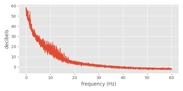
You can read this plot a bit like a histogram, with the frequencies on the x-axis and the rate at which they are present in the signal on the y-axis.
The Nyquist-Shannon sampling theorem tells us that to preserve a given frequency without aliasing we need to sample at at least twice that rate. This is why the x-axis only goes up to 60Hz, even though our signal was sampled at 120Hz - because we can't detect frequencies higher than that.
The y-axis here is in decibels. This is a log-scale quantity where zero does not correspond to anything in-particular - but instead where each 10 ticks corresponds to a 10x reduction in energy.
We can see that there is still energy in the frequencies all the way up to 60Hz, however the majority of the energy is in the frequencies under 30Hz.
That somewhat indicates to me that if at any point we are sampling motion capture data down to anything less than 30Hz, we are very likely to be under-sampling the data and losing information. In this case, either aliasing, over-smoothing, or over-shooting artefacts are basically unavoidable - we just need to pick our poison. If you can't tolerate over-shooting, use a linear filter. If you want something that changes smoothly and don't mind an over-shoot here and there, consider a cubic filter.
The good news is that this graph also indicates that 60Hz is probably not too bad for a lot of motion capture data. And at 60Hz we can likely use filters like lanczos3 with some confidence that they will not produce awful artefacts - both when interpolating a 60Hz signal - and when down-sampling a higher frequency signal to 60Hz. With a higher sample rate than 60Hz we can use even greater window sizes for \( a \), and should expect the aliasing and/or over-shooting artefacts introduced to be fairly minimal. But - as with all such things - your mileage may vary.
Summary
Filtering, Convolutions, Up-Sampling and Down-Sampling are all complicated topics that require a lot of thought. We have a lot of mathematical theory in this domain, but we also have a lot of pragmatic constraints. There is no one-size fits all solution, but here I'll try to summarize some rough advice that I think can help people dealing with mocap data and animation programming to make wise decisions.
How do I apply filters / convolutions to Quaternions?
- Unroll your quaternions. Even though some methods don't require it, it's still almost always better to deal with quaternion signals that don't contain unnecessary discontinuities when doing any kind of signal processing.
- Frame your filtering/convolution operation as a series of weighted sums over local windows of quaternions.
- To compute the weighted sum of quaternions you have three options:
- Fastest: do the weighted sum in the raw quaternion space and re-normalize. Equivalent to a "nlerp".
- Medium: do the weighted sum in the log-space relative to the central quaternion. Equivalent to a "slerp".
- Robust: use the eigen-vector-based method of quaternion averaging.
What sample rate should I use when capturing and processing mocap data offline?
240Hz is probably pretty good for even very fast human motions. If not that, then whatever the highest setting is for your capture device. Try to avoid anything less than 60Hz if possible.
What sample rate should I use when playing back animation data?
Your playback sample rate will be dictated by the sample rate of your game / app / display device. This is usually 60Hz or 30Hz but can vary a lot depending on the user's hardware - both their processing power but also their monitor's refresh rate as many monitors these days have non-standard default refresh rates such as 75Hz.
If your stored data is at a higher sample rate than your display device you should either:
- Down-sample it ahead of time to the rate of the display device using a filter.
- Summarize it on-the-fly to the rate of the display device's using a filter the width of the display device's sampling time.
If your stored data is at an equal or lower sample rate than your display device you should:
- Interpolate it on-the-fly using your chosen filter.
How do I speed-up or slow-down animation data?
This can be considered the same as adjusting for different playback rate, so the advice from above applies here too.
Which filter should I use?
Is avoiding overshoot critical?
Down-Sampling / Summarization: Use a linear or nearest-neighbor filter.
Up-Sampling / Interpolation: Use a linear filter.
Otherwise...
Down-Sampling / Summarization:
- Fastest: Take the nearest-neighbor
- Balanced: Use a 4-frame filter such as a catmull-rom cubic
- Quality: Use a windowed sinc filter such as lanczos3 or larger (at 60Hz or more)
Up-Sampling / Interpolation:
- Fastest: Linear interpolation
- Balanced: Use a 4-frame filter such as catmull-rom cubic
- Quality: Use a windowed sinc filter such as lanczos3 or larger (at 60Hz or more)
How do I reduce sample rate to reduce memory usage?
If you are reducing the sample rate below the rate of your display device in an attempt to save memory then:
Do you know which up-sampling / interpolation method is intended to be used?
- In which case can you optimize for the best down-sampling with respect to that up-sampling method?
If not, or if that is too complicated for your pipeline, down-sample with a filter as normal. If you are down-sampling to 30Hz or less then accept that some amount of aliasing, over-smoothing, or overshoot will be unavoidable.
How do I handle velocities?
Compute the velocities of the input signal and filter those.
What about key-framed animation data?
Is it meant to be hitting exact frames at exact times?
- Leave it alone!
Is it already being interpolated on-the-fly at runtime?
- Treat it like arbitrarily high resolution mocap data.
Conclusion
At the beginning of this article I said that the way most animation programmers handle the temporal aspect of animation data is wrong. Well, this isn't really fair. Because there isn't a "right" way to handle the temporal aspect of animation data - everything is a choice with pros, cons, and tradeoffs.
What is true is that almost all animation software today makes the following choices: linear up-sampling, and nearest-neighbor down-sampling. That's actually a relatively practical choice if you had to make just one context-independent decision. Linear up-sampling is the fastest possible in terms of performance, and nearest-neighbor down-sampling is a perfectly fine choice if you don't mind some aliasing and your animation doesn't contain very high frequencies (which most animation data usually doesn't).
But these are not the best choices in all situations. As I already discussed in my article on cubic interpolation, linear up-sampling has a nasty visual velocity discontinuity. Nearest-neighbor down-sampling can produce aliasing, and makes no attempt to preserve the original signal for some given up-sampling method.
And we don't need to limit ourselves to one context-independent decision. There are contexts where we don't always have to use the most performant and simple up-sampling and down-sampling methods, and there are better ways we can treat our data when we have a bit more understanding of the mathematics involved. All these small differences in the way we treat out data can add up to produce results which are holistically better.
Finally, I'd like to thank Bart Wronski and Marc-André Carbonneau for all their help preparing this article. This is not my area of expertise, and so their input was indispensable. As always, I also welcome any corrections, clarifications, or feedback.
So I hope this article has been even insightful and maybe got you thinking a bit more about up-sampling, down-sampling, and animation data in general. As always, thanks for reading!