Variations on Müller's method of Polar Decomposition
23/11/2024
Today I'd like to talk about one of my favorite techniques in graphics: Müller's method of polar decomposition of 3x3 matrices. I really like this technique because it's a simple and interpretable solution to a problem that you would expect to require some fairly complex linear algebra, and yet it can be implemented in just a few lines of code.
I'd also like to present a couple of variations of Müller's method that I think are useful and interesting, including one which (in my brief experiments at least) seems roughly two times faster to compute, and has a more regular convergence behavior.
If you don't know it, I highly recommend reading the original paper to get an understanding of what Müller's method is and how it works (the paper is quite short and accessible) - but to put it very briefly - it's a method of extracting the rotation part of a 3x3 matrix (generally known as polar decomposition) which works by iteratively trying to find a rotation which rotates a fixed set of basis vectors towards the basis vectors of the matrix we are trying to extract the rotation part from.
Below you can see it in action, with the columns of the matrix we are trying to extract the rotation part from given by the large red green and blue lines, and the resulting orthonormal rotation shown on the small axis and on the duck:
Notably, this method is very stable in the degenerate case, and can be extremely fast if you have a good initial guess. This makes it a great fit for a lot of applications in graphics such as Shape Matching.
The implementation itself is very simple. Here is a version almost identical to the version Müller provides in the paper:
quat quat_muller(mat3 m, quat q0 = quat(), int iterations=30, float eps=1e-8f)
{
    quat q = q0;

    for (int i = 0; i < iterations; i++)
    {
        mat3 r = mat3_from_quat(q);

        vec3 omega = (
            cross(r.c0(), m.c0()) +
            cross(r.c1(), m.c1()) +
            cross(r.c2(), m.c2())) / (fabsf(
            dot(r.c0(), m.c0()) +
            dot(r.c1(), m.c1()) +
            dot(r.c2(), m.c2())) + eps);

        q = quat_mul(quat_from_scaled_angle_axis(omega), q);
    }

    return q;
}
Here, m is the matrix we are trying to extract the rotation part from and q0 is our initial guess - and the result is returned in quaternion form.
One thing to be aware of with this code straight from the paper is that it assumes the matrix we are decomposing has a positive determinant. If the determinant is negative (indicated by grey axes in the previous visualization) it wont converge properly. Making the method generalize to negative determinants is thankfully extremely simple. We just check the determinant, and if it is less than zero we solve for the negation of the matrix m instead.
quat quat_muller_ndet(mat3 m, quat q0 = quat(), int iterations=30, float eps=1e-8f)
{
    if (mat3_det(m) < 0.0f)
    {
        return quat_muller(-m, q0, iterations, eps);
    }
    else
    {
        return quat_muller(m, q0, iterations, eps);
    }
}
So from here on in I'm going to assume the determinant is already positive in all the matrices we are dealing with.
The computational cost of Müller's method is relatively cheap as each iteration only requires a few cross and dot products as well as a couple of trig functions like sin and cos from the quat_from_scaled_angle_axis function (see here). In my experience 30 iterations seems sufficient in almost all cases, and if you have a very good initial guess the number of required iterations could be as low as two or three. If you want to add an early return for convergence, just check if the squared length of omega is less than some small constant and break out of the loop.
The above version is formulated in terms of quaternions, but we can formulate it entirely in terms of matrices too if we prefer:
mat3 mat3_muller(mat3 m, mat3 q0 = mat3(), int iterations=30, float eps=1e-8f)
{
    mat3 q = q0;

    for (int i = 0; i < iterations; i++)
    {
        vec3 omega = (
            cross(q.c0(), m.c0()) +
            cross(q.c1(), m.c1()) +
            cross(q.c2(), m.c2())) / (fabsf(
            dot(q.c0(), m.c0()) +
            dot(q.c1(), m.c1()) +
            dot(q.c2(), m.c2())) + eps);

        q = mat3_mul(mat3_from_scaled_angle_axis(omega), q);
    }

    return q;
}
Here we just need a mat_from_scaled_angle_axis function, which can be implemented using quat_from_scaled_angle_axis:
mat3 mat3_from_scaled_angle_axis(vec3 v)
{
    return mat3_from_quat(quat_from_scaled_angle_axis(v));
}
I've set up a really basic benchmark which runs these two variations on 10000 randomly generated matrices (using 30 iterations) and computes the total time taken divided by 10000. Here are the results:
quat_muller          | 2.562 us
mat3_muller          | 2.603 us
(Standard disclaimer: all this benchmarking should be taken with a grain of salt - I didn't examine the results in any depth at all such as checking the generated assembly or verifying if SIMD instructions are used or not.)
In this benchmark at least, the matrix version is very slightly slower. Presumably this is because the mat3_from_quat function effectively just gets moved inside mat3_from_scaled_angle_axis, and any benefit from more efficient matrix multiplication is offset by the fact we are writing more memory when writing out the result.
In both versions we still have these relatively slow trig functions. Some of you may remember from my article on the exponential map that there is a linear approximation of the from_scaled_angle_axis function which avoids these trig functions. We can see what happens if we use that instead:
quat quat_muller_approx(mat3 m, quat q0 = quat(), int iterations=30, float eps=1e-8f)
{
    quat q = q0;

    for (int i = 0; i < iterations; i++)
    {
        mat3 r = mat3_from_quat(q);

        vec3 omega = (
            cross(r.c0(), m.c0()) +
            cross(r.c1(), m.c1()) +
            cross(r.c2(), m.c2())) / (fabsf(
            dot(r.c0(), m.c0()) +
            dot(r.c1(), m.c1()) +
            dot(r.c2(), m.c2())) + eps);

        q = quat_mul(quat_from_scaled_angle_axis_approx(omega), q);
    }

    return q;
}
Here are the results:
quat_muller          | 2.562 us
mat3_muller          | 2.603 us
quat_muller_approx   | 1.355 us
mat3_muller_approx   | 1.386 us
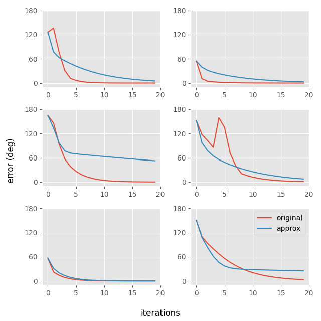
So this runs about twice as fast on a per-iteration basis which is nice... but unfortunately I found that in certain cases it takes an extremely long time to converge. Here is a plot of angular error (against an SVD-based solution) vs iteration count for this version compared to the original on six different randomly generated matrices:

You can see that in some cases it does not appear to converge properly (see middle left or bottom right).
What else can we do here? Well one thing that has always bothered me about Müller's method is that it feels like there should be a way to formulate the required quaternion explicitly rather than going via quat_from_scaled_angle_axis. And in fact there is - but to understand how it works we need to do a little detour and first understand how the quat_between function works.
The quat_between function is a common function in most quaternion libraries which computes the shortest rotation between two vectors. A standard implementation looks like this:
quat quat_between(vec3 p, vec3 q)
{
    vec3 c = cross(p, q);

    return quat_normalize(quat(
        dot(p, q) + sqrtf(dot(p, p) * dot(q, q)),
        c.x,
        c.y,
        c.z));
}
I don't know about you, but to me at least - it is not obvious at all why this works from looking at the code alone. So let me try and explain a little bit...
It starts with the following fact: if we have two vectors and we take the dot product and cross product, and build a quaternion from these two quantities (putting the dot product in the w component, and the cross product in the xyz components), this will give us an (unnormalized) quaternion which rotates arounds the axis perpendicular to the two vectors, by an angle of twice the angle between the two vectors. The reason this is twice the angle is that the w component of the quaternion is defined as the cosine of half the angle of rotation:
quat quat_between_twice(vec3 p, vec3 q)
{
    vec3 c = cross(p, q);

    return quat_normalize(quat(
        dot(p, q),
        c.x,
        c.y,
        c.z));
}
(Aside: It might seem like quat_between_twice is a pretty obscure and useless function, and in many ways it is! But the weirdest thing about it is that it pops up as a somewhat fundamental operation in 3d geometry. I highly recommend this beautiful talk from Freya Holmér if you want to know how and why that is!)
If we want a quaternion which rotates just once the angle between these two vectors we have a couple of options. The first, simplest option is to find the vector which is half way (in terms of angle) between the two vectors we want to rotate between, and use the previous function we defined on this half-way vector instead:
quat quat_between_alt(vec3 p, vec3 q)
{
    vec3 mid = (normalize(p) + normalize(q)) / 2;
    return quat_between_twice(p, mid);
}
But this involves three re-normalizations, so maybe this option is not so great.
The second option is better, but a bit less intuitive. We use the quat_between_twice function as normal, but then we mix the result in equal proportion with the identity quaternion and then re-normalize - to give us a rotation which only rotates half as much.
quat quat_between_alt2(vec3 p, vec3 q)
{
    return quat_normalize(quat_between_twice(p, q) + quat());
}
This still involves two re-normalizations. One way we can get rid of one of these is to mix the identity quaternion with the un-normalized quaternion we get from the dot and cross product. But because this quaternion is un-normalized, it will be proportional in magnitude to the length of p multiplied by the length of q, so we need to scale the identity quaternion we mix it with based on the lengths of p and q too, so the magnitudes match:
quat quat_between_alt3(vec3 p, vec3 q)
{
    vec3 c = cross(p, q);

    quat q0 = quat(dot(p, q), c.x, c.y, c.z);
    quat q1 = quat(sqrtf(dot(p, p)) * sqrtf(dot(q, q)), 0.0f, 0.0f, 0.0f);

    return quat_normalize(q0 + q1);
}
Because the identity quaternion only affects the w component, we can just write this directly inline. And we can remove one of the square roots using the following identity: sqrt(dot(x, x)) * sqrt(dot(y, y)) == sqrt(dot(x, x) * dot(y, y))... which gives us our original formulation back again!
quat quat_between_alt4(vec3 p, vec3 q)
{
    vec3 c = cross(p, q);

    return quat_normalize(quat(
        dot(p, q) + sqrtf(dot(p, p) * dot(q, q)),
        c.x,
        c.y,
        c.z));
}
So effectively all that is happening here is that the cross and dot product are giving us a rotation representing twice the angle we need, and so we are mixing it with the appropriate amount of identity quaternion to reduce it by half.
Now that we understand how quat_between is derived, we can use it to make another variation of Müller's method. The basic idea is this. Instead of using the cross product to get a "torque" which rotates us towards the target, we are going to use the quat_between function to find the three quaternions which rotate us from each of the basis vectors toward the target vectors and then sum/average these quaternions before renormalizing the result.
quat quat_between_unnormalized(vec3 p, vec3 q)
{
    vec3 c = cross(p, q);

    return quat(
        dot(p, q) + sqrtf(dot(p, p) * dot(q, q)),
        c.x,
        c.y,
        c.z);
}

quat quat_muller_var(mat3 m, quat q0 = quat(), int iterations=30, float eps=1e-8f)
{
    quat q = q0;

    for (int i = 0; i < iterations; i++)
    {
        mat3 r = mat3_from_quat(q);

        quat d = quat_normalize(
            quat_between_unnormalized(r.c0(), m.c0()) +
            quat_between_unnormalized(r.c1(), m.c1()) +
            quat_between_unnormalized(r.c2(), m.c2()));

        q = quat_mul(d, q);
    }

    return q;
}
Notice that we sum the unnormalized versions of the quaternions. This helps us in two ways. First, it saves us a few square roots, but more importantly it makes each rotation proportional to the length of the target vector - which is exactly what we want when we compute the "weighted average" of the quaternions.
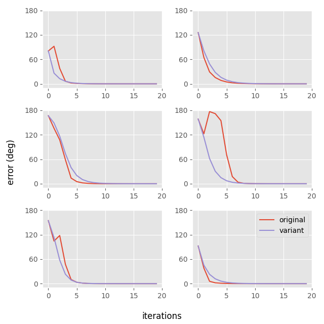
Here is how the convergence of this version looks compared to Müller's original:

We can see that although it occasionally takes more iterations, its behavior is more regular than Müller's original method, where the error can sometimes rise temporarily for the first couple of iterations.
And although it takes more iterations in some cases, this is countered by the fact that this version is faster on a per iteration basis as it does not involved any trig functions:
quat_muller          | 2.562 us
mat3_muller          | 2.603 us
quat_muller_approx   | 1.355 us
mat3_muller_approx   | 1.386 us
quat_muller_var      | 1.489 us
There are some more optimizations we can do too.
We know that the length of p will always be one, since this is the basis vector from the rotation matrix. And we also know that the length of q does not change between iterations so we can compute it once at the beginning and store the result.
quat quat_between_muller_iteration(vec3 p, vec3 q, float qlen)
{
    vec3 c = cross(p, q);

    return quat(
        dot(p, q) + qlen,
        c.x,
        c.y,
        c.z);
}

quat quat_muller_var_alt(mat3 m, quat q0 = quat(), int iterations=30, float eps=1e-8f)
{
    quat q = q0;
    float mc0len = sqrtf(dot(m.c0(), m.c0()));
    float mc1len = sqrtf(dot(m.c1(), m.c1()));
    float mc2len = sqrtf(dot(m.c2(), m.c2()));

    for (int i = 0; i < iterations; i++)
    {
        mat3 r = mat3_from_quat(q);

        quat d = quat_normalize(
            quat_between_muller_iteration(r.c0(), m.c0(), mc0len) +
            quat_between_muller_iteration(r.c1(), m.c1(), mc1len) +
            quat_between_muller_iteration(r.c2(), m.c2(), mc2len));

        q = quat_mul(d, q);
    }

    return q;
}
Then, if we inline quat_between_muller_iteration and expand out the sum, things simplify even more:
quat quat_muller_var_alt2(mat3 m, quat q0 = quat(), int iterations=30, float eps=1e-8f)
{
    quat q = q0;

    float ml =
        sqrtf(dot(m.c0(), m.c0())) +
        sqrtf(dot(m.c1(), m.c1())) +
        sqrtf(dot(m.c2(), m.c2())) + eps;

    for (int i = 0; i < iterations; i++)
    {
        mat3 r = mat3_from_quat(q);

        float w = ml +
            dot(r.c0(), m.c0()) +
            dot(r.c1(), m.c1()) +
            dot(r.c2(), m.c2());

        vec3 v =
            cross(r.c0(), m.c0()) +
            cross(r.c1(), m.c1()) +
            cross(r.c2(), m.c2());

        q = quat_mul(quat_normalize(quat(w, v.x, v.y, v.z)), q);
    }

    return q;
}
I've also added a small epsilon to the sum of the vector lengths. This biases our method towards the identity rotation when the input matrix is zero or close to zero which should help with stability in the degenerate case.
This version with all of our optimizations is faster again in my little benchmark. Now all it has per iteration is a bunch of multiplies, adds, and a single square root to normalize the quaternion. We can also formulate it in terms of matrices if we like:
mat3 mat3_muller_var_alt2(mat3 m, mat3 q0 = mat3(), int iterations=30, float eps=1e-8f)
{
    mat3 q = q0;

    float ml =
        sqrtf(dot(m.c0(), m.c0())) +
        sqrtf(dot(m.c1(), m.c1())) +
        sqrtf(dot(m.c2(), m.c2())) + eps;

    for (int i = 0; i < iterations; i++)
    {
        float w = ml +
            dot(q.c0(), m.c0()) +
            dot(q.c1(), m.c1()) +
            dot(q.c2(), m.c2());

        vec3 v =
            cross(q.c0(), m.c0()) +
            cross(q.c1(), m.c1()) +
            cross(q.c2(), m.c2());

        q = mat3_mul(mat3_from_quat(quat_normalize(quat(w, v.x, v.y, v.z))), q);
    }

    return q;
}
Here is a comparison of the performance of all the different variations:
quat_muller          | 2.562 us
mat3_muller          | 2.603 us
quat_muller_approx   | 1.355 us
mat3_muller_approx   | 1.386 us
quat_muller_var      | 1.489 us
quat_muller_var_alt2 | 1.155 us
mat3_muller_var_alt2 | 1.281 us
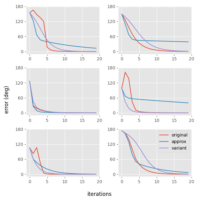
And here is another comparison of the convergence between all the variations which have different convergence behavior on a different set of six random matrices:

Finally, here is a visual comparison between the different methods:
So I think that although it isn't a perfect apples-to-apples comparison it seems like our final version should probably give roughly a 2x improvement on performance compared to Müller's original implementation provided in the paper. Not bad at all!
If you like this article I also wrote about a nice closed-form solution to this very same problem.
Although the method I've presented here works in my experiments, I don't have any kind of proof of convergence or anything like that. From generating random matrices I did not find any case where it failed, but that does not mean there are not pathological edge cases which might somehow break it. This is the problem with getting your code from a blog like mine rather than a peer reviewed paper like Müller's!
Finally, please let me know if this variation already exists and I've just reinvented something already known, so I can add the appropriate citations and references.